Transcriptional phenotyping
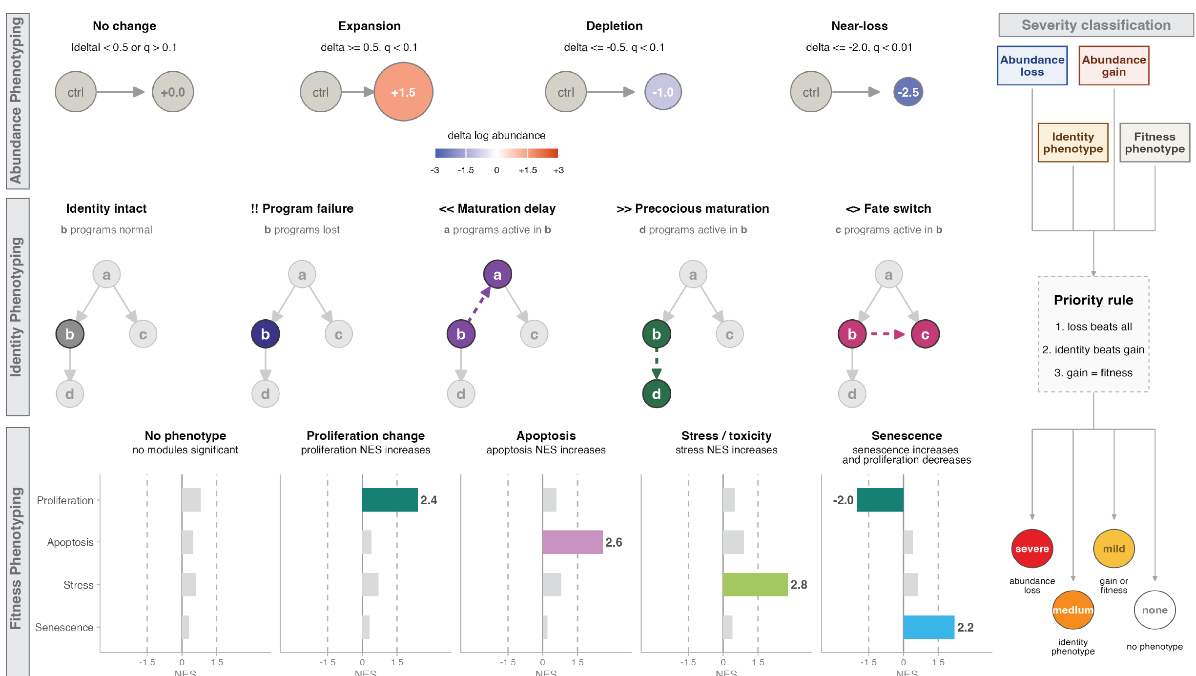
Once we've computed DEGs for a perturbation, the natural next question is: what is the phenotype? Which cell states are genuinely required for a genotype, as opposed to just downstream casualties of some earlier loss? And beyond abundance — is a cell state still present, but not quite itself anymore (delayed, precocious, stressed, or partially misspecified)?
Platt's phenotyping functions turn these per-gene, per-cell-state statistics into calls that summarize an entire perturbation at a glance, and then draw those calls directly on the lineage graph. This replaces the older DvEG (deviantly-expressed genes) workflow, which compared perturbation DEGs against reference DEGs directly — transcriptional phenotyping folds that same question into a broader, graph-topology-aware view of a perturbation's phenotype.
For more information on DEGs, see our Reference DEGs and Perturbation DEGs pages.
Categorizing genetic requirements
The first question to ask of a perturbation is which cell states are lost, and whether that loss is a direct requirement or an indirect consequence of losing an earlier state in the lineage. categorize_genetic_requirements() answers this using the state graph's topology: for each perturbation, it takes the cell states flagged as lost (is_lost_when_present) and looks at where they sit in the lineage. A lost cell state with no lost parent upstream of it in the graph is called directly lost; a lost cell state whose loss can be explained by an already-lost parent is called indirectly lost.
perturb_ccm_tbl- a tibble of fitted genotype models, one row per perturbation, with aperturb_summary_tbllist-column (the per-cell-state loss summary, e.g. from a table offit_genotype_ccm()results)state_graph- anigraphobject describing the lineage relationships among cell states
genetic_requirements = categorize_genetic_requirements(perturb_ccm_tbl, muscle_state_graph@graph)

genetic_requirements %>% head()
| id | perturb_name | perturb_effect |
|---|---|---|
| paraxial mesoderm (tbx16+) | tbx16,msgn1 | direct |
| fast-committed myocyte, pre-fusion | tbx16,msgn1 | indirect |
| fast-committed myocyte, fusing (pcdh7b+) | tbx16,msgn1 | indirect |
In the tbx16-msgn1 crispant, paraxial mesoderm progenitors are directly required — they're lost with no lost parent upstream of them in the graph — while the fast muscle fates downstream are only indirectly lost, as a consequence of losing their progenitor pool.
From impact calls to phenotype glyphs
Abundance loss is only one axis of a phenotype. A cell state can persist in normal numbers and still show a transcriptional identity defect (a maturation delay, a fate switch, a program failure) or fitness-related stress (apoptotic, senescent, or stress-pathway signatures). Platt represents this richer, per-cell-type summary as an impact table — one row per cell type, with categorical calls for abundance, identity, and fitness that are typically assembled upstream from your DEG/DvEG/abundance evidence for a genotype. At minimum, an impact table needs:
cell_type- the cell state being annotatedabundance_code- one of"A0 No change","A1 Expansion","A2 Depletion","A3 Ablation/Loss","A4 Ectopic/extra state"abundance_severity-"none","mild","moderate", or"severe"identity_label- a call describing the transcriptional identity of the state (identity intact, maturation delay, precocious maturation, program failure, fate switch/misspecification, identity fragmentation)fitness_label- a free-text label capturing fitness-related evidence (e.g. mentioning apoptosis, stress, or senescence)
tbx16_impact_table = tibble::tibble(
  cell_type          = c("paraxial mesoderm (tbx16+)",
                          "fast-committed myocyte, pre-fusion",
                          "head and neck mesoderm (pax3+, pax7+)"),
  abundance_code     = c("A3 Ablation/Loss", "A2 Depletion", "A1 Expansion"),
  abundance_severity = c("severe", "moderate", "mild"),
  identity_label     = c("I0 Identity intact", "I3 Program failure within identity", "I0 Identity intact"),
  fitness_label      = c("F2 apoptosis", "none", "none")
)
impact_to_phenos() translates that impact table into the standardized fields the plotting layer expects — an abundance log2FC proxy (from abundance_code x abundance_severity), a compact identity code and glyph string (e.g. "!!" for program failure), and fitness axes for direction, apoptosis, stress score, and senescence:
impact_table- the data frame described abovesev_map- severity label -> magnitude, used to build the abundance proxyabundance_code_map- abundance code -> signed direction/magnitudeidentity_glyph_map- identity label -> glyph string
tbx16_phenos = impact_to_phenos(tbx16_impact_table)

tbx16_phenos %>% select(cell_group, abundance_code, abundance_log2fc, identity_glyph, F2_apoptosis)
You won't usually call impact_to_phenos() directly, though — plot_phenotypes_from_impact() calls it for you as its first step.
Building the impact table automatically, without an LLM
summarize_impact_in_lineage_context() is currently exported from platt's develop_refactor branch only; install that branch (ref = "develop_refactor") to follow this section.
Typing out an impact table by hand only scales to a handful of cell types. For a whole lineage, summarize_impact_in_lineage_context() builds the same table for you — this is the actual function platt's phenotyping pipeline calls, just with llm_fun left at its default of NULL, so no LLM server, Python, or reticulate setup is required. It walks the lineage, joins in your abundance/fitness/identity phenotype calls, pulls out each cell type's significant DEGs and genes-of-interest, and runs pathway enrichment (fgsea::fora(), the same over-representation test used on the Functional Enrichment page) to fill in a disrupted_pathways column.
None of its inputs are typed by hand — each comes from an earlier point in the pipeline:
target_gene_expression- where the perturbation's target gene(s) are actually expressed, filtered down from the reference expression table (expressed in at least 1% of cells, at least 25% as strongly as that gene's own peak expression)dact_results- a differential-abundance-over-time table for the perturbation, reduced to one row per cell type (its peak-effect timepoint)degs- the perturbation's DEG table, e.g.tbx16_degsfrom the Perturbation DEGs pageref_expression- the reference expression tableontologies- a named list ofmsigdbr-style gene set tables, as on the Functional Enrichment pagecombined_psg- thecell_state_graphto traversegenes_of_interest- a regulator/TF panel, e.g. read from a curated regulators tableabundance_phenotypes,fitness_phenotypes,identity_phenotypes- per-cell-type abundance/fitness/identity calls, in the same shape described above but covering the whole graph — produced by an earlier phenotype-assignment step in your pipeline, not written by handllm_fun- a function that asks an LLM to write a short mechanistic summary for each cell type; left at its default ofNULLhere, so this whole step is skipped
tbx16_target_gene_expression = ref_expression %>%
  filter(gene_short_name %in% c("tbx16", "msgn1"), fraction_expressing >= 0.01) %>%
  group_by(gene_short_name) %>%
  mutate(max_expr = max(mean_expression, na.rm = TRUE)) %>%
  ungroup() %>%
  mutate(expr_ratio = mean_expression / max_expr) %>%
  filter(expr_ratio >= 0.25)

tbx16_impact_table_auto = summarize_impact_in_lineage_context(
  target_gene_expression = tbx16_target_gene_expression,
  dact_results           = tbx16_dact_summary_tbl,
  degs                   = tbx16_degs,
  ref_expression         = ref_expression,
  ontologies             = list(BP = gene_set_BP, MF = gene_set_MF, CC = gene_set_CC),
  combined_psg           = muscle_state_graph,
  genes_of_interest      = regulators$gene_short_name,
  abundance_phenotypes   = tbx16_abundance_phenotypes,
  fitness_phenotypes     = tbx16_fitness_phenotypes,
  identity_phenotypes    = tbx16_identity_phenotypes
)
summarize_impact_in_lineage_context() is the same function the full narrative pipeline uses to generate per-cell-type prose (via llm_fun) — passing llm_fun = NULL is the "null model": no LLM server, Python, or reticulate setup required, just the deterministic abundance/identity/fitness calls and pathway enrichment. tbx16_impact_table_auto has the same required columns as the hand-typed tbx16_impact_table above (plus DEG/pathway columns impact_to_phenos() ignores), so it drops into impact_to_phenos() / plot_phenotypes_from_impact() the same way — just built from real pipeline data across the whole graph instead of three rows typed by hand.
Plotting phenotype calls on the graph
plot_phenotypes_from_impact() is the entrypoint you'll reach for most often: hand it your cell_state_graph and an impact table, and it converts the table with impact_to_phenos() and renders the annotated lineage graph in one call:
cell_state_graph- a plattcell_state_graphobjectimpact_table- the impact table described aboveshow_node_labels- label the cell states...- additional arguments forwarded toplot_phenotypes_glyphs()
plot_phenotypes_from_impact(muscle_state_graph,
                            tbx16_impact_table,
                            show_node_labels = TRUE)
Each node's fill encodes the abundance call (expansion, depletion, or ablation/loss), and a short bold glyph is drawn on top of the node to encode the identity call — "" for identity intact, "<<" for a maturation delay, ">>" for precocious maturation, "!!" for a program failure within identity, "<>" for a fate switch or misspecification, and "##" for identity fragmentation. In the tbx16-msgn1 crispant above, paraxial mesoderm progenitors are lost outright, while the fast-committed myocytes that do persist show a program-failure glyph ("!!") — consistent with the depleted pax3a signal we saw on the Perturbation DEGs page.
If you want more control over the plot — for instance, restricting to a subset of cell types, or tuning label sizes — you can call plot_phenotypes_glyphs() directly on a table you've already run through impact_to_phenos():
cell_state_graph- a plattcell_state_graphobjectphenos_df- a phenotype table, typically fromimpact_to_phenos()map- a named list mapping the phenotype roles (lfc,q,ident,glyph,f1-f4) to columns inphenos_dfnode_overlay-"glyphs"(the default) to draw the identity glyphs on each node, or"none"to suppress themcell_types- restrict the plot to a subset of cell statesshow_node_labels- ifTRUEandlabel_cell_typesis left unset, label every node
plot_phenotypes_glyphs(muscle_state_graph,
                       tbx16_phenos,
                       cell_types = c("paraxial mesoderm (tbx16+)",
                                      "fast-committed myocyte, pre-fusion"),
                       show_node_labels = TRUE)
For more information on plotting Platt graphs more generally, see our plotting page.