Clustering and classifying your cells
Single-cell experiments are often performed on tissues containing many cell
types. Monocle 3 provides a simple set of functions you can use to group your
cells according to their gene expression profiles into
In this section, you will learn how to cluster cells using Monocle 3. We will
demonstrate the main functions used for clustering with the
You can load the data into Monocle 3 like this:
library(monocle3)
library(dplyr) # imported for some downstream data manipulation

expression_matrix <- readRDS(url("https://depts.washington.edu:/trapnell-lab/software/monocle3/celegans/data/cao_l2_expression.rds"))
cell_metadata <- readRDS(url("https://depts.washington.edu:/trapnell-lab/software/monocle3/celegans/data/cao_l2_colData.rds"))
gene_annotation <- readRDS(url("https://depts.washington.edu:/trapnell-lab/software/monocle3/celegans/data/cao_l2_rowData.rds"))

cds <- new_cell_data_set(expression_matrix,
                         cell_metadata = cell_metadata,
                         gene_metadata = gene_annotation)
Pre-process the data
Now that the data's all loaded up, we need to
cds <- preprocess_cds(cds, num_dim = 100)
It's a good idea to check that you're using enough PCs to capture most of
the variation in gene expression across all the cells in the data set. You
can look at the fraction of variation explained by each PC using
plot_pc_variance_explained():
plot_pc_variance_explained(cds)
We can see that using more than 100 PCs would capture only a small amount of additional variation, and each additional PC makes downstream steps in Monocle slower.
Reduce dimensionality and visualize the cells
Now we're ready to visualize the cells. To do so, you can use either
t-SNE,
which is very popular in single-cell RNA-seq, or UMAP,
which is increasingly common. Monocle 3 uses UMAP by default, as we feel that it is both faster and better suited for
clustering and trajectory analysis in RNA-seq. To reduce the dimensionality of the data down into the X, Y plane so
we can plot it easily, call reduce_dimension():
cds <- reduce_dimension(cds)To plot the data, use Monocle's main plotting function, plot_cells():
plot_cells(cds)
Each point in the plot above represents a different cell in the cell_data_set
object cds. As you can see the cells form many groups, some with thousands of
cells, some with only a few. Cao & Packer annotated each cell according to type manually by looking
at which genes it expresses. We can color the cells in the UMAP plot by the authors' original annotations
using the color_cells_by argument to plot_cells().
plot_cells(cds, color_cells_by="cao_cell_type")
You can see that many of the cell types land very close to one another in the UMAP plot.
Except for a few cases described in a moment, color_cells_by can be the name of any column in
colData(cds). Note that when color_cells_by is a categorical variable, labels are
added to the plot, with each label positioned roughly in the middle of all the cells that have that label.
You can also color your cells according to how much of a gene or set of genes they express:
plot_cells(cds, genes=c("cpna-2", "egl-21", "ram-2", "inos-1"))
Faster clustering with UMAP
If you have a relatively large dataset (with >10,000 cells or more), you may want to take advantage
of options that can accelerate UMAP. Passing umap.fast_sgd=TRUE to
reduce_dimension() will use a fast stochastic gradient descent method inside of UMAP.
If your computer has multiple cores, you can use the cores argument to make UMAP multithreaded.
However, invoking reduce_dimension() with either of these options will make it produce slighly
different output each time you run it. If this is acceptable to you, you could see signifant reductions in
the running time of reduction_dimension().
If you want, you can also use t-SNE to visualize your data. First, call reduce_dimension with
reduction_method="tSNE".
cds <- reduce_dimension(cds, reduction_method="tSNE")Then, when you call plot_cells(), pass reduction_method="tSNE" to it as well:
plot_cells(cds, reduction_method="tSNE", color_cells_by="cao_cell_type")
You can actually use UMAP and t-SNE on the same cds object - one won't overwrite the results of the
other. But you must specify which one you want in downstream functions like plot_cells.

Check for and remove batch effects
When performing gene expression analysis, it's important to check for
You should always check for batch effects when you perform dimensionality reduction. You should add a column to
the colData that encodes which batch each cell is from. Then you can simply color the cells by batch.
Cao & Packer et al included a "plate" annotation in their data, which specifies which sci-RNA-seq plate each cell
originated from. Coloring the UMAP by plate reveals:
plot_cells(cds, color_cells_by="plate", label_cell_groups=FALSE)
Dramatic batch effects are not evident in this data. If the data contained more substantial variation due to plate, we'd expect to see groups of cells that really only come from one plate. Nevertheless, we can try and remove what batch effect is by running the align_cds() function:
cds <- align_cds(cds, num_dim = 100, alignment_group = "plate")
cds <- reduce_dimension(cds)
plot_cells(cds, color_cells_by="plate", label_cell_groups=FALSE)
When run with the alignment_group argument, align_cds() tries to remove batch effects using mutual nearest neighbor alignment, a technique introduced by John Marioni's lab. Monocle 3 does so by calling Aaron Lun's excellent package batchelor. If you use align_cds(), be sure to call get_citations() to see how you should cite the software on which Monocle depends.

Group cells into clusters
Grouping cells into clusters is an important step in identifying the cell types represented in your data. Monocle uses a technique called community detection to group cells. This approach was introduced by Levine et al as part of the phenoGraph algorithm. You can cluster your cells using the cluster_cells() function, like this:
cds <- cluster_cells(cds, resolution=1e-5)
plot_cells(cds)
Note that now when we call plot_cells() with no arguments, it colors the cells by
cluster according to default.
The cluster_cells() also divides the cells into larger, more well separated groups called
plot_cells(cds, color_cells_by="partition", group_cells_by="partition")
Once you run cluster_cells(), the plot_cells() function will label each cluster of cells
is labeled separately according to how you want to color the cells. For example, the call below colors the cells
according to their cell type annotation, and each cluster is labeled according the most common annotation within it:
plot_cells(cds, color_cells_by="cao_cell_type")
You can choose to label whole partitions instead of clusters by passing group_cells_by="partition".
You can also plot the top 2 labels per cluster by passing labels_per_group=2 to plot_cells().
Finally, you can disable this labeling policy, making plot_cells() behave like it did before we called
cluster_cells(), like this:
plot_cells(cds, color_cells_by="cao_cell_type", label_groups_by_cluster=FALSE)
Find marker genes expressed by each cluster
Once cells have been clustered, we can ask what genes makes them different from one another. To do that, start by calling
the
marker_test_res <- top_markers(cds, group_cells_by="partition",
                               reference_cells=1000, cores=8)
The data frame marker_test_res contains a number of metrics for how specifically expressed each gene
is in each partition. We could group the cells according to cluster, partition, or any categorical variable in
colData(cds). You can rank the table according to one or more of the specificity metrics and take the top
gene for each cluster. For example, pseudo_R2 is one such measure. We can rank markers according to
pseudo_R2 like this:
top_specific_markers <- marker_test_res %>%
                            filter(fraction_expressing >= 0.10) %>%
                            group_by(cell_group) %>%
                            top_n(1, pseudo_R2)

top_specific_marker_ids <- unique(top_specific_markers %>% pull(gene_id))
Now, we can plot the expression and fraction of cells that express each marker in each group with the
plot_genes_by_group function:
plot_genes_by_group(cds,
                    top_specific_marker_ids,
                    group_cells_by="partition",
                    ordering_type="maximal_on_diag",
                    max.size=3)
It's often informative to look at more than one marker, which you can do just by changing the first argument to
top_n():
top_specific_markers <- marker_test_res %>%
                            filter(fraction_expressing >= 0.10) %>%
                            group_by(cell_group) %>%
                            top_n(3, pseudo_R2)

top_specific_marker_ids <- unique(top_specific_markers %>% pull(gene_id))

plot_genes_by_group(cds,
                    top_specific_marker_ids,
                    group_cells_by="partition",
                    ordering_type="cluster_row_col",
                    max.size=3)
There are many ways to compare and contrast clusters (and other groupings) of cells. We will explore them in great detail in the differential expression analysis section a bit later.
Annotate your cells according to type
Identifying the type of each cell in your dataset is critical for many downstream analyses. There are several ways of
doing this. One commonly used approach is to first cluster the cells and then assign a cell type to each cluster based
on its gene expression profile. We've already seen how to use top_markers(). Reviewing literature associated
with a marker gene often give strong indications of the identity of clusters that express it. In Cao & Packer
colData(cds)$cao_cell_type.
To assign cell types based on clustering, we begin by creating a new column in colData(cds) and
initialize it with the values of partitions(cds) (can also use clusters(cds) depending on your dataset):
colData(cds)$assigned_cell_type <- as.character(partitions(cds))
Now, we can use the dplyrpackage's recode() function to
remap each cluster to a different cell type:
colData(cds)$assigned_cell_type <- dplyr::recode(colData(cds)$assigned_cell_type,
                                                 "1"="Body wall muscle",
                                                 "2"="Germline",
                                                 "3"="Motor neurons",
                                                 "4"="Seam cells",
                                                 "5"="Sex myoblasts",
                                                 "6"="Socket cells",
                                                 "7"="Marginal_cell",
                                                 "8"="Coelomocyte",
                                                 "9"="Am/PH sheath cells",
                                                 "10"="Ciliated neurons",
                                                 "11"="Intestinal/rectal muscle",
                                                 "12"="Excretory gland",
                                                 "13"="Chemosensory neurons",
                                                 "14"="Interneurons",
                                                 "15"="Unclassified eurons",
                                                 "16"="Ciliated neurons",
                                                 "17"="Pharyngeal gland cells",
                                                 "18"="Unclassified neurons",
                                                 "19"="Chemosensory neurons",
                                                 "20"="Ciliated neurons",
                                                 "21"="Ciliated neurons",
                                                 "22"="Inner labial neuron",
                                                 "23"="Ciliated neurons",
                                                 "24"="Ciliated neurons",
                                                 "25"="Ciliated neurons",
                                                 "26"="Hypodermal cells",
                                                 "27"="Mesodermal cells",
                                                 "28"="Motor neurons",
                                                 "29"="Pharyngeal gland cells",
                                                 "30"="Ciliated neurons",
                                                 "31"="Excretory cells",
                                                 "32"="Amphid neuron",
                                                 "33"="Pharyngeal muscle")
Let's see how the new annotations look:
plot_cells(cds, group_cells_by="partition", color_cells_by="assigned_cell_type")
Partition 7 has some substructure, and it's not obvious just from looking at the output of top_markers()
what cell type or types it corresponds to. So we can isolate it with the choose_cells() function for
further analysis:
cds_subset <- choose_cells(cds)
Now we have a smaller cell_data_set object that contains just the cells from the partition we'd like to
drill into. We can use graph_test() to identify genes that are differentially expressed in different
subsets of cells from this partition:
pr_graph_test_res <- graph_test(cds_subset, neighbor_graph="knn", cores=8)
pr_deg_ids <- row.names(subset(pr_graph_test_res, morans_I > 0.01 & q_value < 0.05))
We will learn more about graph_test() in the
differential expression analysis
section later. We can take all the genes that vary across this set of cells and group those that have similar patterns
of expression into
gene_module_df <- find_gene_modules(cds_subset[pr_deg_ids,], resolution=1e-3)Plotting these modules' aggregate expression values reveals which cells express which modues.
plot_cells(cds_subset, genes=gene_module_df,
           show_trajectory_graph=FALSE,
           label_cell_groups=FALSE)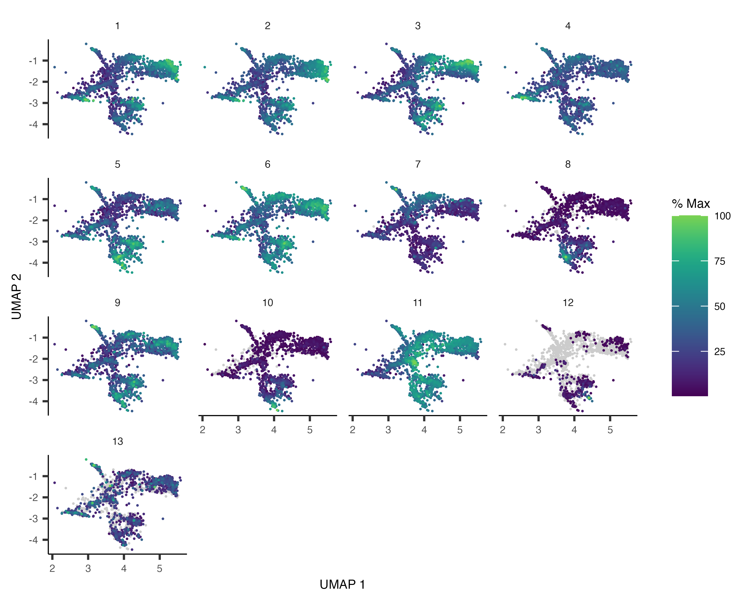
You can explore the genes in each module or conduct gene ontology enrichment analysis on them to glean insights about which cell types are present. Suppose after doing this we have a good idea of what the cell types in the partition are. Let's recluster the cells at finer resolution and then see how they overlap with the clusters in the partition:
cds_subset <- cluster_cells(cds_subset, resolution=1e-2)
plot_cells(cds_subset, color_cells_by="cluster")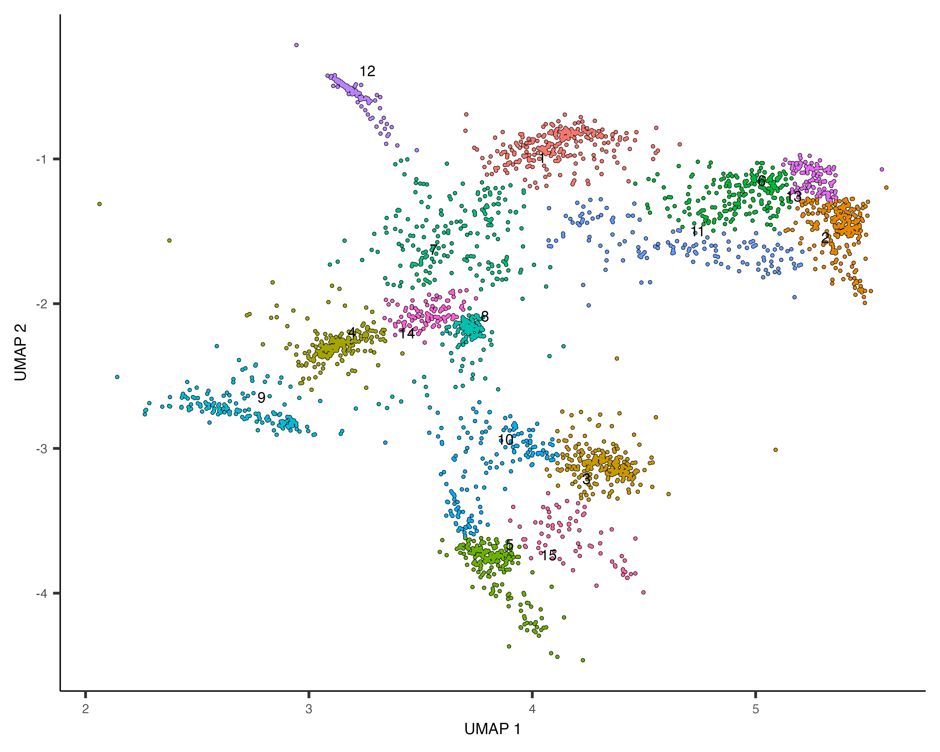
Based on how the patterns line up, we'll make the following assignments:
colData(cds_subset)$assigned_cell_type <- as.character(clusters(cds_subset)[colnames(cds_subset)])
colData(cds_subset)$assigned_cell_type <- dplyr::recode(colData(cds_subset)$assigned_cell_type,
                                                        "1"="Sex myoblasts",
                                                        "2"="Somatic gonad precursors",
                                                        "3"="Vulval precursors",
                                                        "4"="Sex myoblasts",
                                                        "5"="Vulval precursors",
                                                        "6"="Somatic gonad precursors",
                                                        "7"="Sex myoblasts",
                                                        "8"="Sex myoblasts",
                                                        "9"="Ciliated neurons",
                                                        "10"="Vulval precursors",
                                                        "11"="Somatic gonad precursor",
                                                        "12"="Distal tip cells",
                                                        "13"="Somatic gonad precursor",
                                                        "14"="Sex myoblasts",
                                                        "15"="Vulval precursors")

plot_cells(cds_subset, group_cells_by="cluster", color_cells_by="assigned_cell_type")
Now we can transfer the annotations from the cds_subset object back to the full dataset. We'll also filter
out low-quality cells at this stage
colData(cds)[colnames(cds_subset),]$assigned_cell_type <- colData(cds_subset)$assigned_cell_type
cds <- cds[,colData(cds)$assigned_cell_type != "Failed QC" | is.na(colData(cds)$assigned_cell_type )]
plot_cells(cds, group_cells_by="partition",
           color_cells_by="assigned_cell_type",
           labels_per_group=5)
Automated annotation with Garnett
The above process for manually annotating cells by type can be laborious, and must be re-done if the underlying cluster changes. We recently developed Garnett, a software toolkit for automatically annotating cells. Garnett classifies cells based on marker genes. If you've gone through the trouble of annotated your cells manually, Monocle can generate a file of marker genes that can be used with Garnett. This will help you annotate other datasets in the future or reannotate this one if you refine your analysis and update your clustering in the future.
To generate a Garnett file, first find the top markers that each annotated cell type expresses:
assigned_type_marker_test_res <- top_markers(cds,
                                             group_cells_by="assigned_cell_type",
                                             reference_cells=1000,
                                             cores=8)
Next, filter these markers according to how stringent you want to be:
# Require that markers have at least JS specificty score > 0.5 and
# be significant in the logistic test for identifying their cell type:
garnett_markers <- assigned_type_marker_test_res %>%
                        filter(marker_test_q_value < 0.01 & specificity >= 0.5) %>%
                        group_by(cell_group) %>%
                        top_n(5, marker_score)
# Exclude genes that are good markers for more than one cell type:
garnett_markers <- garnett_markers %>%
                        group_by(gene_short_name) %>%
                        filter(n() == 1)
Then call generate_garnett_marker_file:
generate_garnett_marker_file(garnett_markers, file="./marker_file.txt")generate_garnett_marker_file
> Cell type Ciliated sensory neurons
expressed: che-3, scd-2, C33A12.4, R102.2, F27C1.11

> Cell type Non-seam hypodermis
expressed: col-14, col-180, F11E6.3, grsp-1, C06A8.3

> Cell type Seam cells
expressed: col-65, col-77, col-107, ram-2, Y47D7A.13

> Cell type Vulval precursors
expressed: col-68, col-145, lin-31, osm-11, Y62E10A.19

> Cell type Body wall muscle
expressed: csq-1, hum-9, cpna-2, tag-278, F41C3.5

> Cell type Coelomocytes
expressed: cup-4, inos-1, Y73F4A.1, ZC116.3, aman-1

> Cell type flp-1 interneurons
expressed: daf-10, flp-1, nlp-10, zig-2, H05L03.3

> Cell type Sex myoblasts
expressed: egl-15, C04E12.2

> Cell type Intestinal/rectal muscle
expressed: egl-20, lbp-2, bgal-1, ttr-10, T23B12.8

> Cell type Am/PH sheath cells
expressed: far-8, F35B12.9, ZK822.4, F20A1.1, T02B11.3

> Cell type Oxygen sensory neurons
expressed: flp-17, gcy-9, gcy-33, ist-1, Y57G11B.97

> Cell type Pharyngeal neurons
expressed: flr-2, nlp-6, F14B6.2, degt-1, flp-28

> Cell type Unclassified neurons
expressed: gar-2, madd-4, twk-49

> Cell type Germline
expressed: gld-1, pgl-1, ppw-2, prg-2, cbd-1

> Cell type Somatic gonad precursors
expressed: inx-9, mnm-2, C36B7.4

> Cell type Touch receptor neurons
expressed: mec-1, mec-7, mec-12, mec-17, mec-18

> Cell type Pharyngeal epithelia
expressed: pgp-14, pqn-74, fipr-2, R03C1.1, Y73F4A.2

> Cell type Pharyngeal muscle
expressed: pqn-29, F31D4.5, R13H4.8, T01B7.8, T20B6.3

> Cell type Pharyngeal gland
expressed: F15A4.6, dod-6, C49G7.3, M04G7.1, phat-4

> Cell type Canal associated neurons
expressed: acbp-6, Y66D12A.14, ZC412.4, C32E8.6, C41A3.1
The marker files produced by generate_garnett_marker_file() are just a starting point for classifying your
cells with Garnett. You may want to edit this file to add or remove markers based on literature or other information. You
also should consider defining subtypes of cells, which can greatly increase the usefulness and accuracy of Garnett. For
example, the L2 data contains many different types of neurons. Making a "Neuron" cell type in the file above and then using
the subtype of keyword to organize the various subtypes of neurons will make Garnett more able to recognize
them and distinguish them from non-neuronal cell types. When two or more of your cell types share most of their top markers
in plot_genes_by_group(), consider defining a broader cell type definition of which they are both subtypes.
You might also want to define markers for the various subtypes of neurons by subsetting the cds object above
and running top_markers() just on them. See the Garnett
documentation for more on how you can enrich your marker
files.
When you're ready run Garnett, load the package:
Garnett for Monocle 3
Garnett was originally written to work with Monocle 2. We have created a branch of Garnett that works with Monocle 3, which will eventually replace the main branch. In the meantime, you must install and load the Monocle 3 branch of Garnett!
## Install the monocle3 branch of garnett
BiocManager::install(c("org.Mm.eg.db", "org.Hs.eg.db"))
devtools::install_github("cole-trapnell-lab/garnett", ref="monocle3")library(garnett)
# install gene database for worm
BiocManager::install("org.Ce.eg.db")Now train a Garnett classifier based on your marker file like this:
colData(cds)$garnett_cluster <- clusters(cds)
worm_classifier <- train_cell_classifier(cds = cds,
                                         marker_file = "./marker_file.txt",
                                         db=org.Ce.eg.db::org.Ce.eg.db,
                                         cds_gene_id_type = "ENSEMBL",
                                         num_unknown = 50,
                                         marker_file_gene_id_type = "SYMBOL",
                                         cores=8)
Now that we've trained a classifier worm_classifier, we can use it to annotate the L2 cells according to type:
cds <- classify_cells(cds, worm_classifier,
                      db = org.Ce.eg.db::org.Ce.eg.db,
                      cluster_extend = TRUE,
                      cds_gene_id_type = "ENSEMBL")
Here's how Garnett annotated the cells:
plot_cells(cds,
           group_cells_by="partition",
           color_cells_by="cluster_ext_type")
Garnett classifiers can be applied to datasets other than the one they were trained on. We strongly encourage you to share your Garnett files and include them with your papers so that others can use them.
As part of writing a paper about Garnett, we trained a Garnett model to classify classify_cells()
function:
ceWhole <- readRDS(url("https://cole-trapnell-lab.github.io/garnett/classifiers/ceWhole_20191017.RDS"))
cds <- classify_cells(cds, ceWhole,
                      db = org.Ce.eg.db,
                      cluster_extend = TRUE,
                      cds_gene_id_type = "ENSEMBL")