Project a query data set onto a reference data set
Co-embedding is used to compare similar data sets in order to identify similarities and differences and transfer annotations between cells. When the data sets are large and there are many sets to compare, the memory and run time requirements for processing co-embedded data can become impediments. Monocle3's solution is to save the models that transform a reference data set to low-dimensional PCA and UMAP space, and then use the models to transform query data sets to the low-dimensional reference space where one can plot them for comparison or annotate query cells by finding similar reference cells.
Load the reference and query data sets
We begin by loading the reference and query data sets into Monocle3. To simplify this example, we load both data sets together; however, one can process them independently.
library(monocle3)
library(Matrix)

# Load the reference data set.
matrix_ref <- readMM(gzcon(url("https://depts.washington.edu:/trapnell-lab/software/monocle3/mouse/data/cao.mouse_embryo.sample.mtx.gz")))
cell_ann_ref <- read.csv(gzcon(url("https://depts.washington.edu:/trapnell-lab/software/monocle3/mouse/data/cao.mouse_embryo.sample.coldata.txt.gz"), text=TRUE), sep='\t')
gene_ann_ref <- read.csv(gzcon(url("https://depts.washington.edu:/trapnell-lab/software/monocle3/mouse/data/cao.mouse_embryo.sample.rowdata.txt.gz"), text=TRUE), sep='\t')

cds_ref <- new_cell_data_set(matrix_ref,
                             cell_metadata = cell_ann_ref,
                             gene_metadata = gene_ann_ref)

# Load the query data set.
matrix_qry <- readMM(gzcon(url("https://depts.washington.edu:/trapnell-lab/software/monocle3/mouse/data/srivatsan.mouse_embryo_scispace.sample.mtx.gz")))
cell_ann_qry <- read.csv(gzcon(url("https://depts.washington.edu:/trapnell-lab/software/monocle3/mouse/data/srivatsan.mouse_embryo_scispace.sample.coldata.txt.gz"), text=TRUE), sep='\t')
gene_ann_qry <- read.csv(gzcon(url("https://depts.washington.edu:/trapnell-lab/software/monocle3/mouse/data/srivatsan.mouse_embryo_scispace.sample.rowdata.txt.gz"), text=TRUE), sep='\t')

cds_qry <- new_cell_data_set(matrix_qry,
                             cell_metadata = cell_ann_qry,
                             gene_metadata = gene_ann_qry)
Remove genes that are not in both data sets
It is essential that the query cds has the same genes in the same order as the reference cds, so we identify the shared genes and sort them.
# Genes in reference.
genes_ref <- row.names(cds_ref)

# Genes in query.
genes_qry <- row.names(cds_qry)

# Shared genes.
genes_shared <- intersect(genes_ref, genes_qry)

# Remove non-shared genes.
cds_ref <- cds_ref[genes_shared,]
cds_qry <- cds_qry[genes_shared,]
Apply a common UMI cutoff
We filter the cells by applying the same UMI cutoff to our data sets. For these data sets, we applied a cutoff of 1000 to reduce their sizes but we show how to find these cutoffs.
# Reference data set UMI cutoff.
numi_ref <- min(colData(cds_ref)[['Total_mRNAs']])
# numi_ref is 1001
numi_qry <- min(colData(cds_qry)[['n.umi']])
# numi_qry is 1000
Estimate size factors
After applying the gene and UMI filters, we re-calculate the size factors of both data sets.
cds_ref <- estimate_size_factors(cds_ref)
cds_qry <- estimate_size_factors(cds_qry)
Process the reference data set
We are ready to process the reference data set by transforming it into PCA and and UMAP low dimension spaces. By setting the build_nn_index to TRUE, we build a nearest neighbor index in the UMAP space, which we will use to transfer the reference annotations to the query. After processing, we save the transform models and nearest neighbor index so that we can use them to transform the query data set into the reference space.
cds_ref <- preprocess_cds(cds_ref, num_dim=100)
cds_ref <- reduce_dimension(cds_ref, build_nn_index=TRUE)
# Save the PCA and UMAP transform models for use with projection.
save_transform_models(cds_ref, 'cds_ref_test_models')
Project the query data set into the reference space
We loaded and filtered the query data into cds_qry earlier in this example so now we load the reference transform models into cds_qry using the load_transform_models() function. load_transform_models() can read reference models stored in a directory created using either store_transform_models() or save_monocle_objects(). Either way, load_transform_models() loads only the transform models into cds_qry. We project the query data into the reference space using the preprocess_transform() and reduce_dimension_transform() functions.
# Load the reference transform models into the query cds.
cds_qry <- load_transform_models(cds_qry, 'cds_ref_test_models')
# Apply the reference transform models to the query cds.
cds_qry <- preprocess_transform(cds_qry)
cds_qry <- reduce_dimension_transform(cds_qry)
Plot the combined data sets
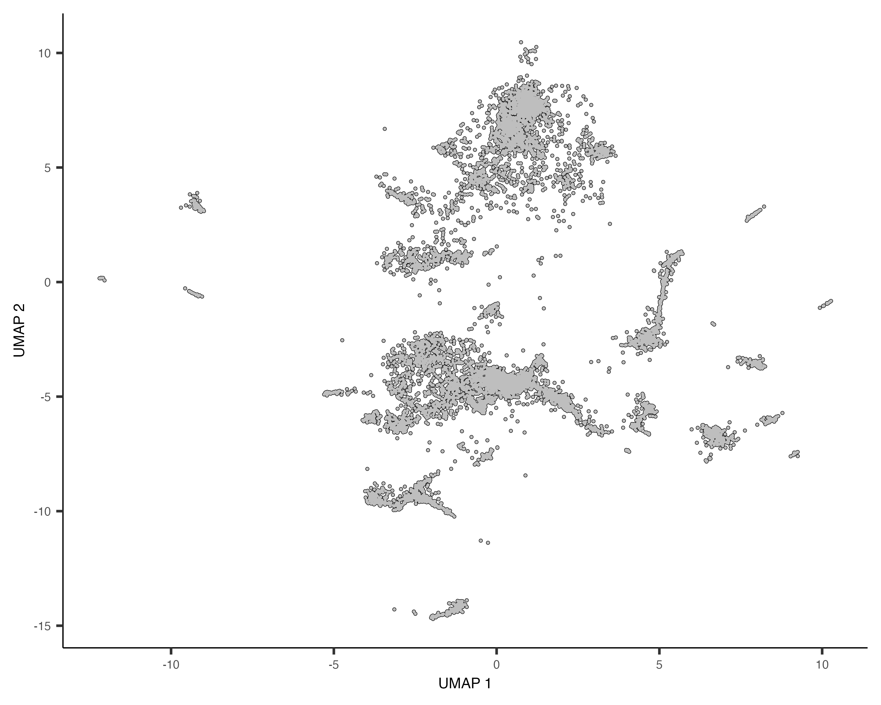
First we plot the reference and query cells in UMAP space.
plot_cells(cds_ref)
plot_cells(cds_qry)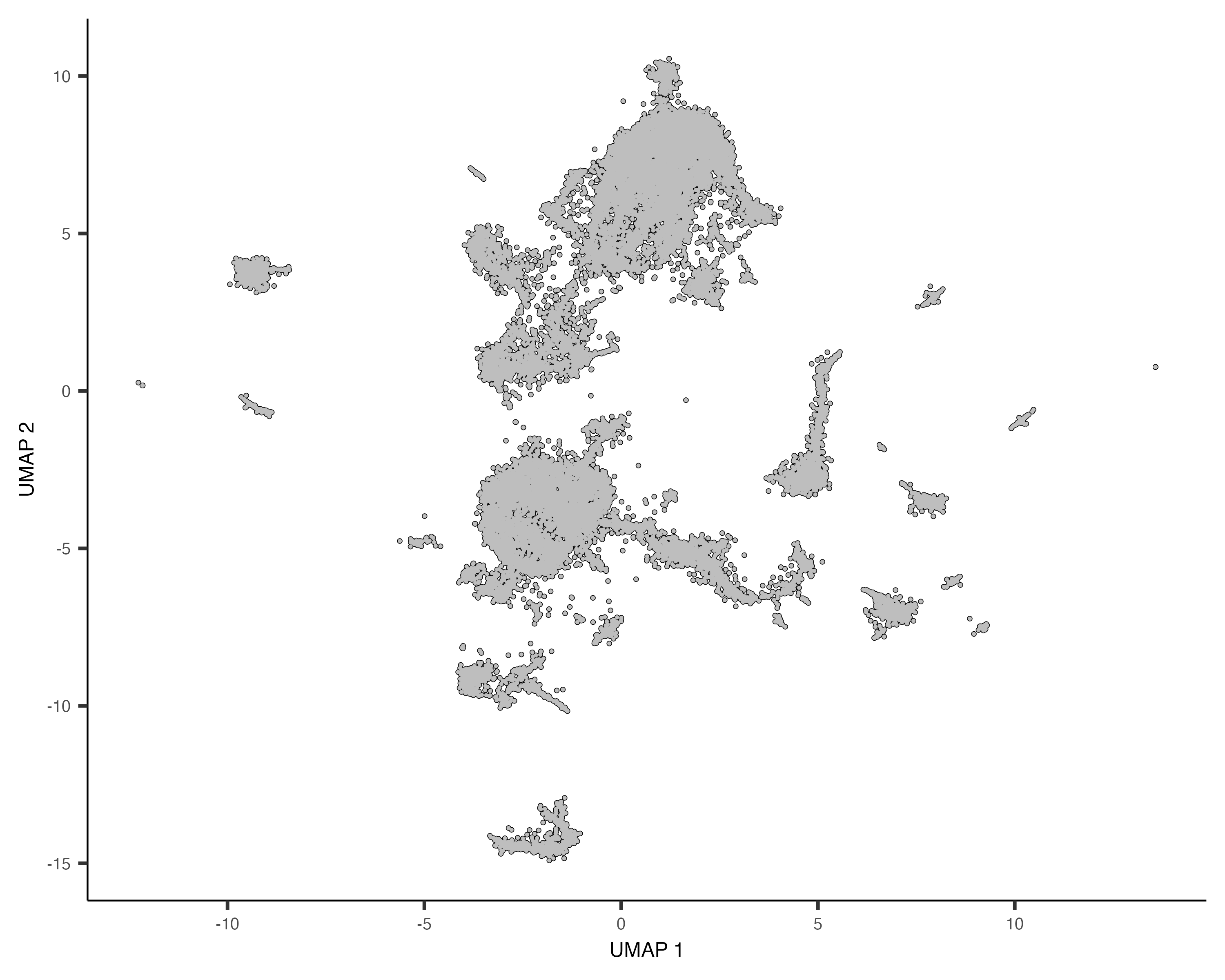
Plot the combined data sets
Now we label the cells in the reference and query cdses, combine the cdses, and plot the combined cells.
# Label the data sets.
colData(cds_ref)[['data_set']] <- 'reference'
colData(cds_qry)[['data_set']] <- 'query'
# Combine the reference and query data sets.
cds_combined <- combine_cds(list(cds_ref, cds_qry),  keep_all_genes=TRUE, cell_names_unique=TRUE, keep_reduced_dims=TRUE)
plot_cells(cds_combined, color_cells_by='data_set')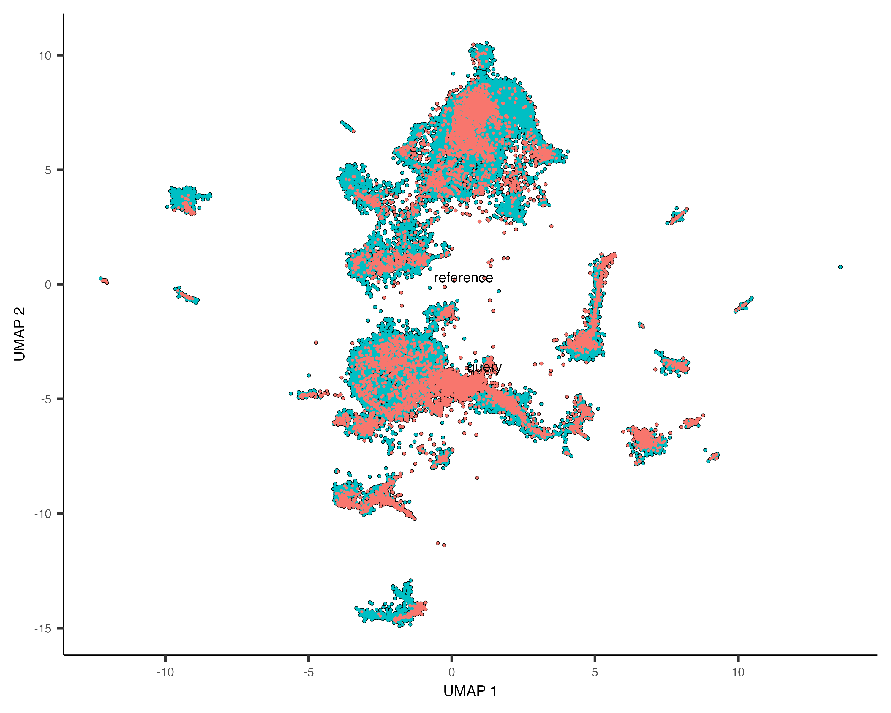
Transfer the reference cell labels to the query data set
Now we transfer the cell type annotations from the reference to the query data set using the nearest neighbor index that we made in the reference UMAP space.
cds_qry_lab_xfr <- transfer_cell_labels(cds_qry, reduction_method='UMAP', ref_coldata=colData(cds_ref), ref_column_name='Main_cell_type', query_column_name='cell_type_xfr', transform_models_dir='cds_ref_test_models')
cds_qry_lab_fix <- fix_missing_cell_labels(cds_qry_lab_xfr, reduction_method='UMAP', from_column_name='cell_type_xfr', to_column_name='cell_type_fix')