Getting started with Monocle 3
Workflow steps at a glance
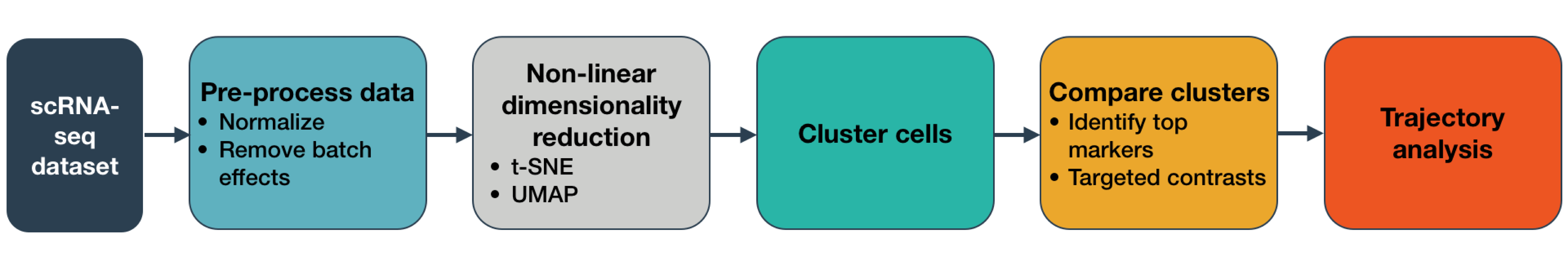
Below, you can see snippets of code that highlight the main steps of Monocle 3. Click on the section headers to jump to the detailed sections describing each one and allowing you to try the steps on example data.
Store data in a cell_data_set object
The first step in working with Monocle 3 is to load up your data into Monocle 3's main class,cell_data_set:
cds <- new_cell_data_set(expression_matrix,
                         cell_metadata = cell_metadata,
                         gene_metadata = gene_annotation)

## Step 1: Normalize and pre-process the data
cds <- preprocess_cds(cds, num_dim = 100)
Optional Remove batch effects
You can subtracted unwatched batch effects or align cells from similar (but not exactly) the same conditions using several different methods in Monocle 3.## Step 2: Remove batch effects with cell alignment
cds <- align_cds(cds, alignment_group = "batch")Cluster your cells
You can easily cluster your cells to find new types:## Step 3: Reduce the dimensions using UMAP
cds <- reduce_dimension(cds)
## Step 4: Cluster the cells
cds <- cluster_cells(cds)Optional Order cells in pseudotime along a trajectory
Now, put your cells in order by how much progress they've made through whatever process you're studying, such as differentiation, reprogramming, or an immune response.## Step 5: Learn a graph
cds <- learn_graph(cds)
## Step 6: Order cells
cds <- order_cells(cds)
plot_cells(cds)Optional Perform differential expression analysis
Compare groups of cells in myriad ways to find differentially expressed genes, controlling for batch effects and treatments as you like:# With regression:
gene_fits <- fit_models(cds, model_formula_str = "~embryo.time")
fit_coefs <- coefficient_table(gene_fits)
emb_time_terms <- fit_coefs %>% filter(term == "embryo.time")
emb_time_terms <- emb_time_terms %>% mutate(q_value = p.adjust(p_value))
sig_genes <- emb_time_terms %>% filter (q_value < 0.05) %>% pull(gene_short_name)
# With graph autocorrelation:
pr_test_res <- graph_test(cds, neighbor_graph="principal_graph", cores=4)
pr_deg_ids <- row.names(subset(pr_test_res, q_value < 0.05))Get started
Load Monocle 3
library(monocle3)

# The tutorial shown below and on subsequent pages uses two additional packages:
library(ggplot2)
library(dplyr)
Loading your data
Monocle 3 takes as input cell by gene expression matrix. Monocle 3 is designed for use with absolute transcript counts (e.g. from UMI experiments). Monocle 3 works "out-of-the-box" with the transcript count matrices produced by Cell Ranger, the software pipeline for analyzing experiments from the 10X Genomics Chromium instrument. Monocle 3 also works well with data from other RNA-Seq workflows such as sci-RNA-Seq and instruments like the Biorad ddSEQ.The cell_data_set class
Monocle holds single-cell expression data in objects of thecell_data_set class. The class is derived from the Bioconductor
SingleCellExperiment class,
which provides a common interface familiar to those who have analyzed other
single-cell experiments with Bioconductor. The class requires three input files:
-
expression_matrix, a numeric matrix of expression values, where rows are genes, and columns are cells -
cell_metadata, a data frame, where rows are cells, and columns are cell attributes (such as cell type, culture condition, day captured, etc.) -
gene_metadata, an data frame, where rows are features (e.g. genes), and columns are gene attributes, such as biotype, gc content, etc.
Required dimensions for input files
- have the same number of columns as the
cell_metadatahas rows. - have the same number of rows as the
gene_metadatahas rows.
- row names of the
cell_metadataobject should match the column names of the expression matrix. - row names of the
gene_metadataobject should match row names of the expression matrix. - one of the columns of the
gene_metadatashould be named "gene_short_name", which represents the gene symbol or simple name (generally used for plotting) for each gene.
Generate a cell_data_set
You can create a new cell_data_set (CDS) object as follows:
# Load the data
expression_matrix <- readRDS(url("https://depts.washington.edu:/trapnell-lab/software/monocle3/celegans/data/cao_l2_expression.rds"))
cell_metadata <- readRDS(url("https://depts.washington.edu:/trapnell-lab/software/monocle3/celegans/data/cao_l2_colData.rds"))
gene_annotation <- readRDS(url("https://depts.washington.edu:/trapnell-lab/software/monocle3/celegans/data/cao_l2_rowData.rds"))


# Make the CDS object
cds <- new_cell_data_set(expression_matrix,
                         cell_metadata = cell_metadata,
                         gene_metadata = gene_annotation)
Generate a cell_data_set from 10X output
To input data from 10X Genomics Cell Ranger, you can use the
load_cellranger_data function:
Note: load_cellranger_data takes an argument umi_cutoff
that determines how many reads a cell must have to be included. By default, this is set to 100.
If you would like to include all cells, set umi_cutoff to 0.
For load_cellranger_data to find the correct files, you must provide a path to the folder containing the
un-modified Cell Ranger 'outs' folder. Your file structure should look like: 10x_data/outs/filtered_feature_bc_matrix/
where filtered_feature_bc_matrix contains files features.tsv.gz, barcodes.tsv.gz and matrix.mtx.gz.
(load_cellranger_data can also handle Cell Ranger V2 data where "features" is substituted for "gene" and
the files are not gzipped.)
# Provide the path to the Cell Ranger output.
cds <- load_cellranger_data("~/Downloads/10x_data")
Alternatively, you can use load_mm_data to load any data in MatrixMarket format by providing the matrix files
and two metadata files (features information and cell information). For more details, run ?load_mm_data
cds <- load_mm_data(mat_path = "~/Downloads/matrix.mtx",
                    feature_anno_path = "~/Downloads/features.tsv",
                    cell_anno_path = "~/Downloads/barcodes.tsv")
Working with large data sets
Some single-cell RNA-Seq experiments report measurements from tens of thousands of cells or more. As instrumentation improves and costs drop, experiments will become ever larger and more complex, with many conditions, controls, and replicates. A matrix of expression data with 50,000 cells and a measurement for each of the 25,000+ genes in the human genome can take up a lot of memory. However, because current protocols typically don't capture all or even most of the mRNA molecules in each cell, many of the entries of expression matrices are zero. Using sparse matrices can help you work with huge datasets on a typical computer. We generally recommend the use of sparse matrices for most users, as it speeds up many computations even for more modestly sized datasets.
To work with your data in a sparse format, simply provide it to Monocle 3
as a sparse matrix from the Matrix package:
cds <- new_cell_data_set(as(umi_matrix, "sparseMatrix"),
cell_metadata = cell_metadata,
gene_metadata = gene_metadata)
Don't accidentally convert to a dense expression matrix
new_cell_data_set without first converting it to a
dense matrix (via as.matrix(), because that may exceed your
available memeory.
Matrix package.
Other sparse matrix packages, such as slam or
SparseM are not supported.
Combining CDS objects
If you have multiple CDS objects that you would like to analyze together, use our
combine_cds. combine_cds takes a list of CDS objects and
combines them into a single CDS object.
# make a fake second cds object for demonstration
cds2 <- cds[1:100,]

big_cds <- combine_cds(list(cds, cds2))
Options
keep_all_genes: When TRUE (default), all genes are kept even if they don't match
between the different CDSs. Cells that do not have a given gene in their CDS will
be marked as having zero expression. When FALSE, only the genes in common among all
CDSs will be kept.
cell_names_unique: When FALSE (default), the cell names in the CDSs are not
assumed to be unique, and so a CDS specifier is appended to each cell name. When TRUE,
no specifier is added.