Constructing single-cell trajectories

During development, in response to stimuli, and throughout life, cells transition from one functional "state" to another. Cells in different states express different sets of genes, producing a dynamic repetoire of proteins and metabolites that carry out their work. As cells move between states, they undergo a process of transcriptional re-configuration, with some genes being silenced and others newly activated. These transient states are often hard to characterize because purifying cells in between more stable endpoint states can be difficult or impossible. Single-cell RNA-Seq can enable you to see these states without the need for purification. However, to do so, we must determine where each cell is in the range of possible states.

Monocle introduced the strategy of using RNA-Seq for single-cell trajectory analysis. Rather than purifying cells into discrete states experimentally, Monocle uses an algorithm to learn the sequence of gene expression changes each cell must go through as part of a dynamic biological process. Once it has learned the overall "trajectory" of gene expression changes, Monocle can place each cell at its proper position in the trajectory. You can then use Monocle's differential analysis toolkit to find genes regulated over the course of the trajectory, as described in the section Finding genes that change as a function of pseudotime . If there are multiple outcomes for the process, Monocle will reconstruct a "branched" trajectory. These branches correspond to cellular "decisions", and Monocle provides powerful tools for identifying the genes affected by them and involved in making them. You can see how to analyze branches in the section Analyzing branches in single-cell trajectories .

The workflow for reconstructing trajectories is very similar to the workflow for clustering, but it has a few additional steps. To illustrate the workflow, we will use another C. elegans data set, this one from Packer & Zhu et al. Their study includes a time series analysis of whole developing embyros. We will examine a small subset of the data which includes most of the neurons. We will load it as we did with the L2 data:

expression_matrix <- readRDS(url("https://depts.washington.edu:/trapnell-lab/software/monocle3/celegans/data/packer_embryo_expression.rds"))
cell_metadata <- readRDS(url("https://depts.washington.edu:/trapnell-lab/software/monocle3/celegans/data/packer_embryo_colData.rds"))
gene_annotation <- readRDS(url("https://depts.washington.edu:/trapnell-lab/software/monocle3/celegans/data/packer_embryo_rowData.rds"))

cds <- new_cell_data_set(expression_matrix,
                         cell_metadata = cell_metadata,
                         gene_metadata = gene_annotation)

Pre-process the data

Pre-processing works exactly as in clustering analysis. This time, we will use a different strategy for batch correction, which includes what Packer & Zhu et al did in their original analysis:

Note: Your data will not have the loading batch information demonstrated here, you will correct batch using your own batch information.

cds <- preprocess_cds(cds, num_dim = 50)
cds <- align_cds(cds, alignment_group = "batch", residual_model_formula_str = "~ bg.300.loading + bg.400.loading + bg.500.1.loading + bg.500.2.loading + bg.r17.loading + bg.b01.loading + bg.b02.loading")

Note that in addition to using the alignment_group argument to align_cds(), which aligns groups of cells (i.e. batches), we are also using residual_model_formula_str. This argument is for subtracting continuous effects. You can use this to control for things like the fraction of mitochondrial reads in each cell, which is sometimes used as a QC metric for each cell. In this experiment (as in many scRNA-seq experiments), some cells spontanously lyse, releasing their mRNAs into the cell suspension immediately prior to loading into the single-cell library prep. This "supernatant RNA" contaminates each cells' transcriptome profile to a certain extent. Fortunately, it is fairly straightforward to estimate the level of background contamination in each batch of cells and subtract it, which is what Packer et al did in the original study. Each of the columns bg.300.loading, bg.400.loading, corresponds to a background signal that a cell might be contaminated with. Passing these colums as terms in the residual_model_formula_str tells align_cds() to subtract these signals prior to dimensionality reduction, clustering, and trajectory inference. Note that you can call align_cds() with alignment_group, residual_model_formula, or both.

Reduce dimensionality and visualize the results

Next, we reduce the dimensionality of the data. However, unlike clustering, which works well with both UMAP and t-SNE, here we strongly urge you to use UMAP, the default method:

cds <- reduce_dimension(cds)
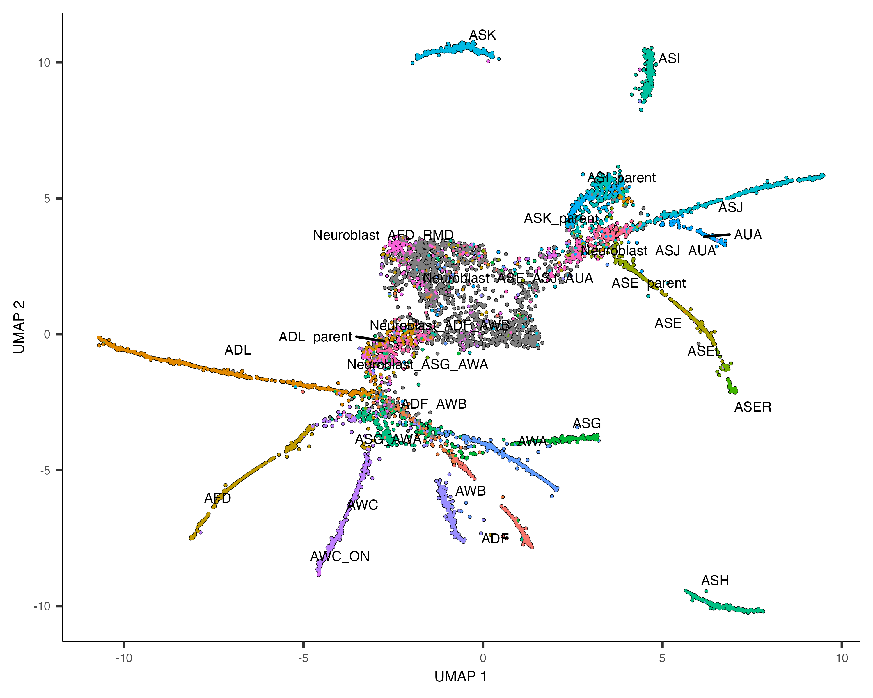
plot_cells(cds, label_groups_by_cluster=FALSE,  color_cells_by = "cell.type")

As you can see, despite the fact that we are only looking at a small slice of this dataset, Monocle reconstructs a trajectory with numerous branches. Overlaying the manual annotations on the UMAP reveals that these branches are principally occupied by one cell type.

As with clustering analysis, you can use plot_cells() to visualize how individual genes vary along the trajectory. Let's look at some genes with interesting patterns of expression in ciliated neurons:

ciliated_genes <- c("che-1",
                    "hlh-17",
                    "nhr-6",
                    "dmd-6",
                    "ceh-36",
                    "ham-1")

plot_cells(cds,
           genes=ciliated_genes,
           label_cell_groups=FALSE,
           show_trajectory_graph=FALSE)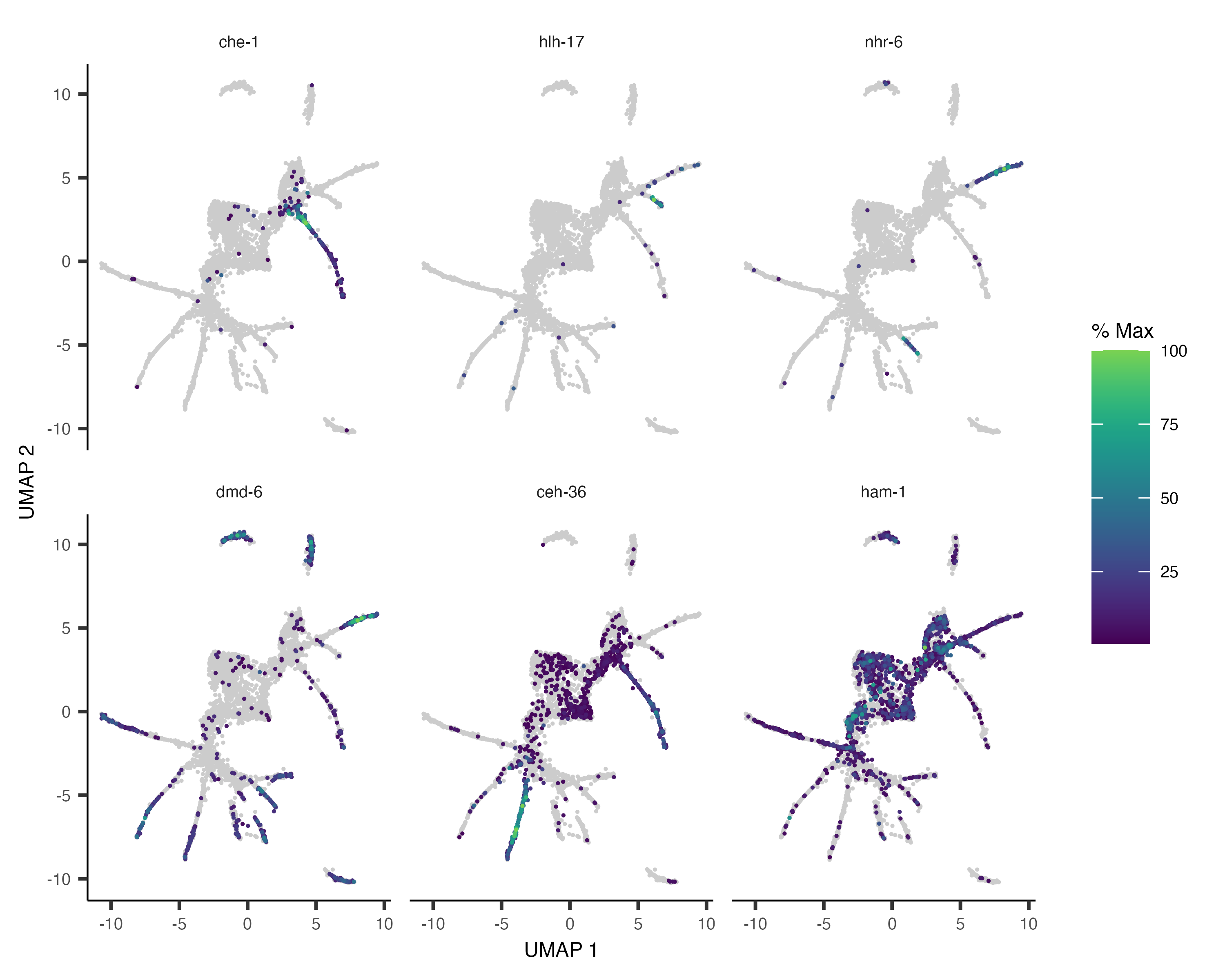

We will learn how to identify the genes that are restricted to each outcome of the trajectory later on in the section Finding genes that change as a function of pseudotime.

Cluster your cells

Although cells may continuously transition from one state to the next with no discrete boundary between them, Monocle does not assume that all cells in the dataset descend from a common transcriptional "ancestor". In many experiments, there might in fact be multiple distinct trajectories. For example, in a tissue responding to an infection, tissue resident immune cells and stromal cells will have very different initial transcriptomes, and will respond to infection quite differently, so they should be a part of the same trajectory.

Monocle is able to learn when cells should be placed in the same trajectory as opposed to separate trajectories through its clustering procedure. Recall that we run cluster_cells(), each cell is assigned not only to a cluster but also to a partition. When you are learning trajectories, each partition will eventually become a separate trajectory. We run cluster_cells()as before.

cds <- cluster_cells(cds)
plot_cells(cds, color_cells_by = "partition")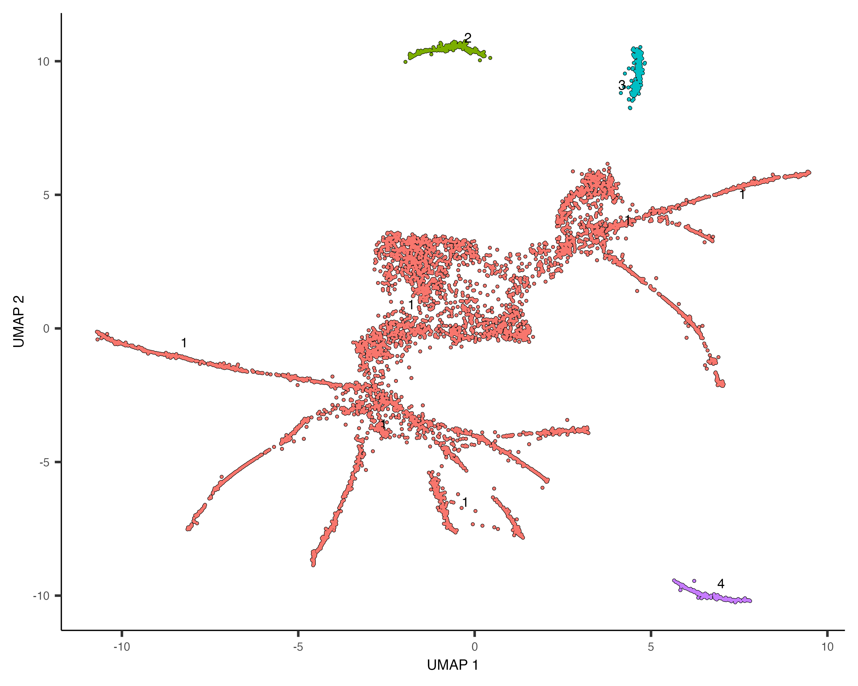

Learn the trajectory graph

Next, we will fit a principal graph within each partition using the learn_graph() function:

cds <- learn_graph(cds)
plot_cells(cds,
           color_cells_by = "cell.type",
           label_groups_by_cluster=FALSE,
           label_leaves=FALSE,
           label_branch_points=FALSE)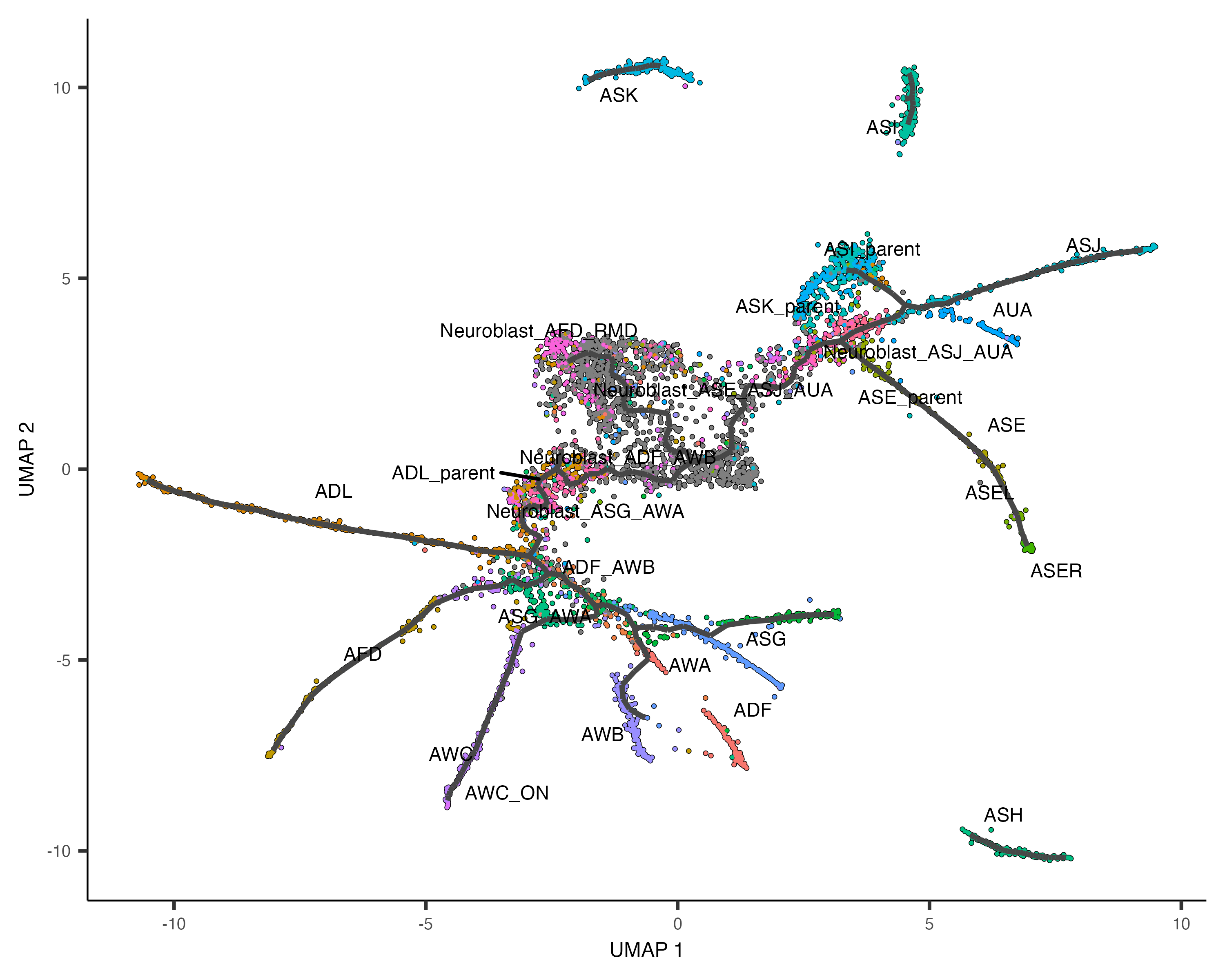

This graph will be used in many downstream steps, such as branch analysis and differential expression.

Order the cells in pseudotime

Once we've learned a graph, we are ready to order the cells according to their progress through the developmental program. Monocle measures this progress in pseudotime. The box below defines pseudotime.

In order to place the cells in order, we need to tell Monocle where the "beginning" of the biological process is. We do so by choosing regions of the graph that we mark as "roots" of the trajectory. In time series experiments, this can usually be accomplished by finding spots in the UMAP space that are occupied by cells from early time points:

plot_cells(cds,
           color_cells_by = "embryo.time.bin",
           label_cell_groups=FALSE,
           label_leaves=TRUE,
           label_branch_points=TRUE,
           graph_label_size=1.5)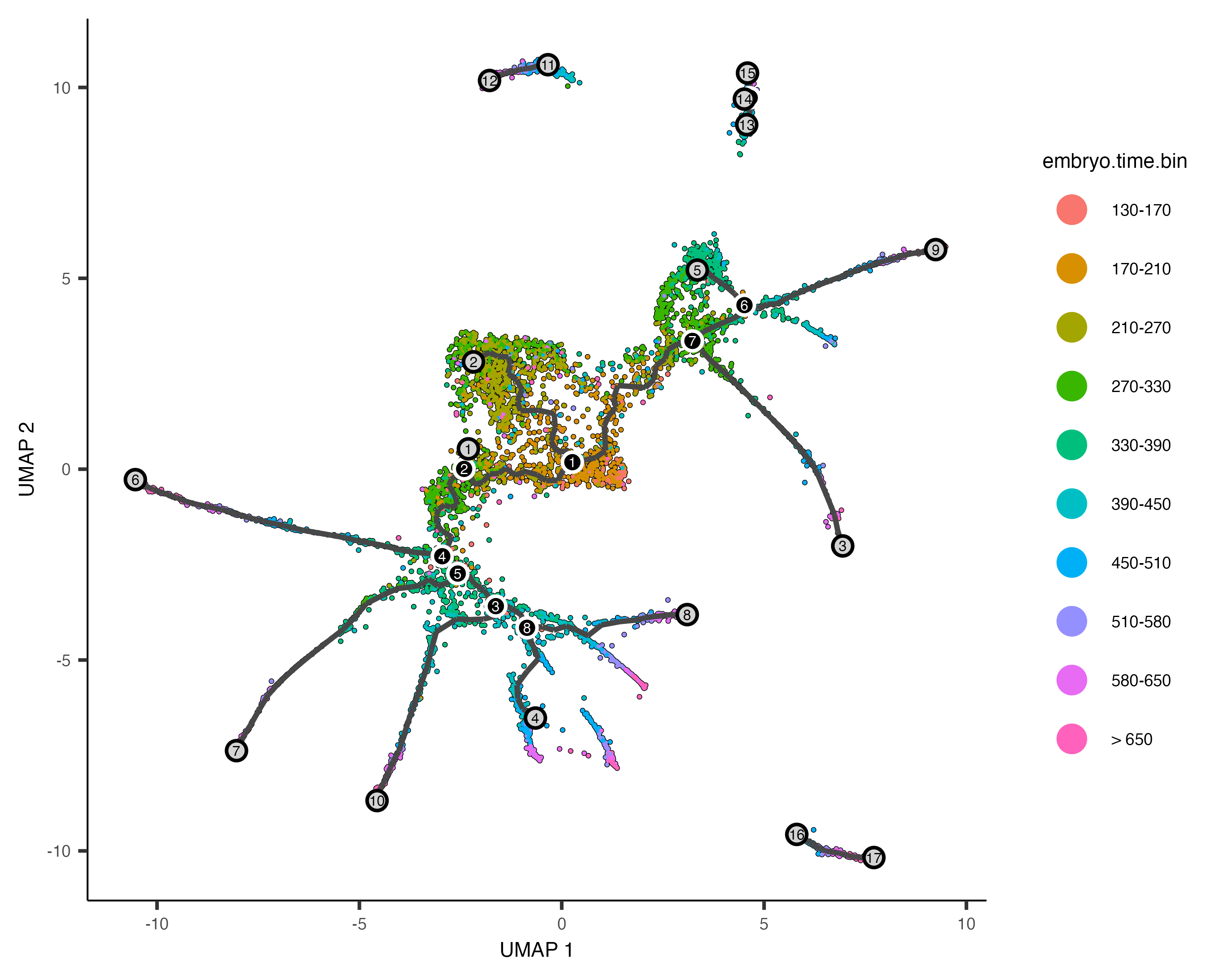

The black lines show the structure of the graph. Note that the graph is not fully connected: cells in different partitions are in distinct components of the graph. The circles with numbers in them denote special points within the graph. Each leaf, denoted by light gray circles, corresponds to a different outcome (i.e. cell fate) of the trajectory. Black circles indicate branch nodes, in which cells can travel to one of several outcomes. You can control whether or not these are shown in the plot with the label_leaves and label_branch_points arguments to plot_cells. Please note that numbers within the circles are provided for reference purposes only.

Now that we have a sense of where the early cells fall, we can call order_cells(), which will calculate where each cell falls in pseudotime. In order to do so order_cells()needs you to specify the root nodes of the trajectory graph. If you don't provide them as an argument, it will launch a graphical user interface for selecting one or more root nodes.

cds <- order_cells(cds)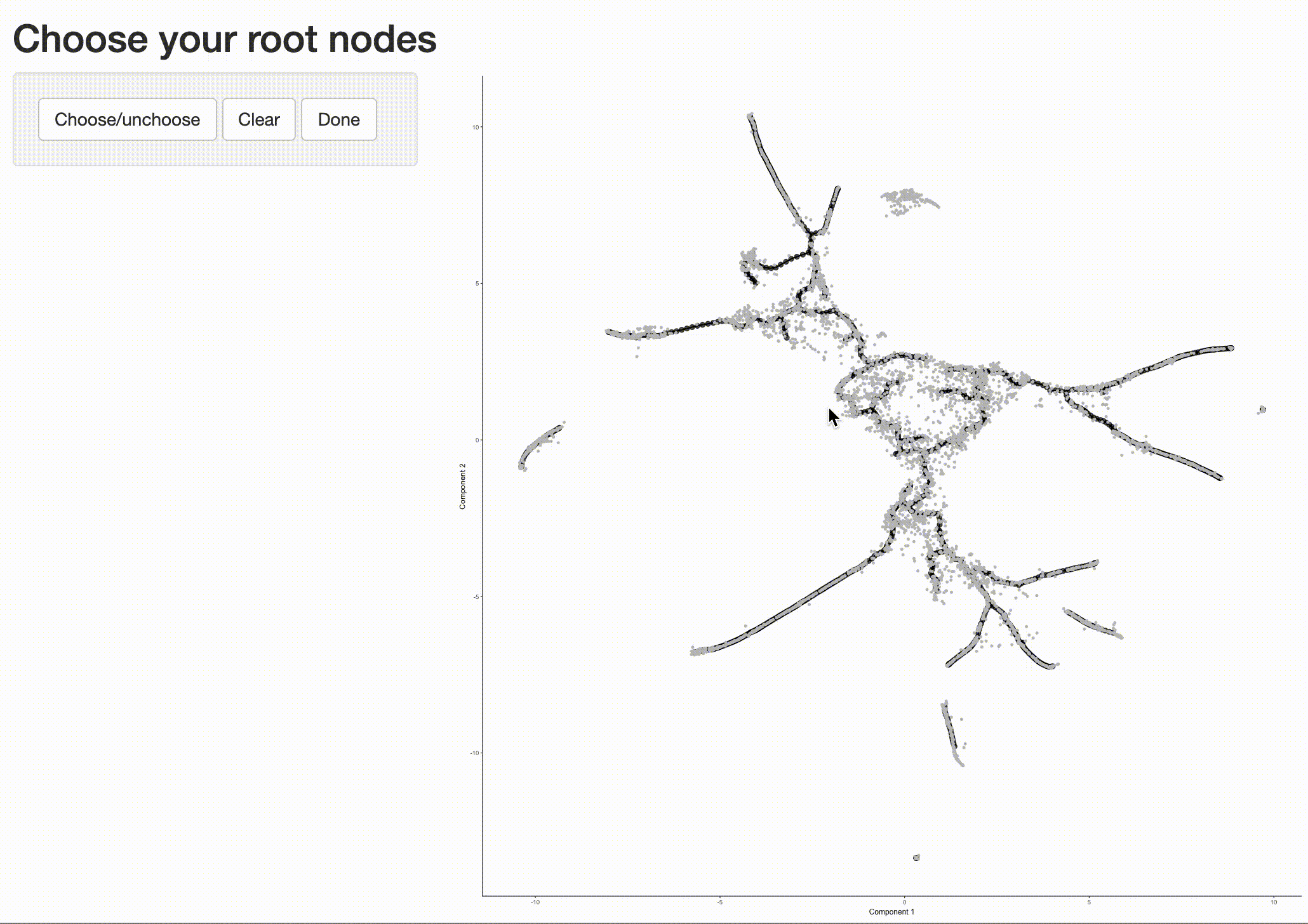

In the above example, we just chose one location, but you could pick as many as you want. Plotting the cells and coloring them by pseudotime shows how they were ordered:

plot_cells(cds,
           color_cells_by = "pseudotime",
           label_cell_groups=FALSE,
           label_leaves=FALSE,
           label_branch_points=FALSE,
           graph_label_size=1.5)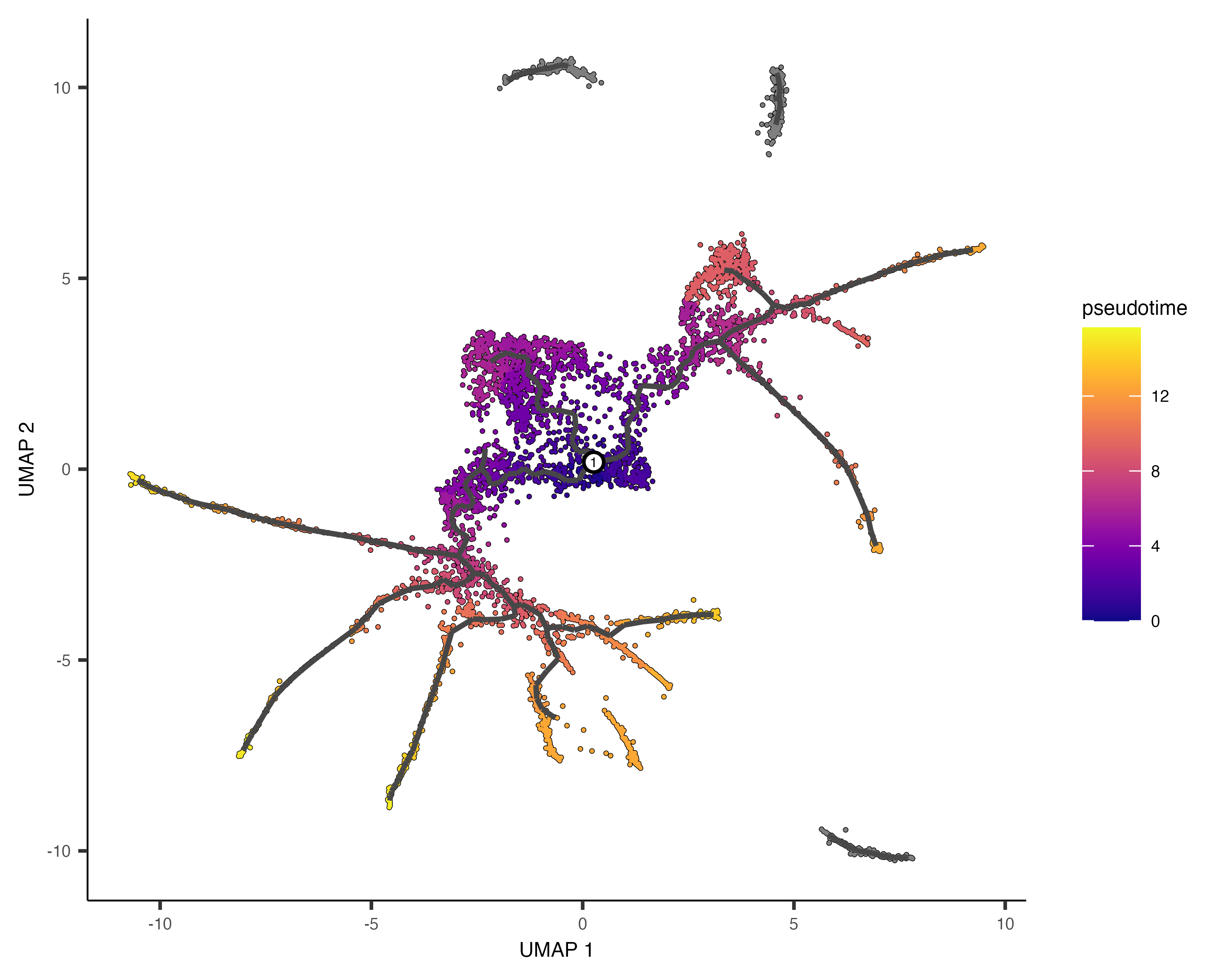

Note that some of the cells are gray. This means they have infinite pseudotime, because they were not reachable from the root nodes that were picked. In general, any cell on a partition that lacks a root node will be assigned an infinite pseudotime. In general, you should choose at least one root per partition.

It's often desirable to specify the root of the trajectory programmatically, rather than manually picking it. The function below does so by first grouping the cells according to which trajectory graph node they are nearest to. Then, it calculates what fraction of the cells at each node come from the earliest time point. Then it picks the node that is most heavily occupied by early cells and returns that as the root.

# a helper function to identify the root principal points:
get_earliest_principal_node <- function(cds, time_bin="130-170"){
  cell_ids <- which(colData(cds)[, "embryo.time.bin"] == time_bin)
  
  closest_vertex <-
  cds@principal_graph_aux[["UMAP"]]$pr_graph_cell_proj_closest_vertex
  closest_vertex <- as.matrix(closest_vertex[colnames(cds), ])
  root_pr_nodes <-
  igraph::V(principal_graph(cds)[["UMAP"]])$name[as.numeric(names
  (which.max(table(closest_vertex[cell_ids,]))))]
  
  root_pr_nodes
}
cds <- order_cells(cds, root_pr_nodes=get_earliest_principal_node(cds))

Passing the programatically selected root node to order_cells() via the root_pr_nodeargument yields:

plot_cells(cds,
           color_cells_by = "pseudotime",
           label_cell_groups=FALSE,
           label_leaves=FALSE,
           label_branch_points=FALSE,
           graph_label_size=1.5)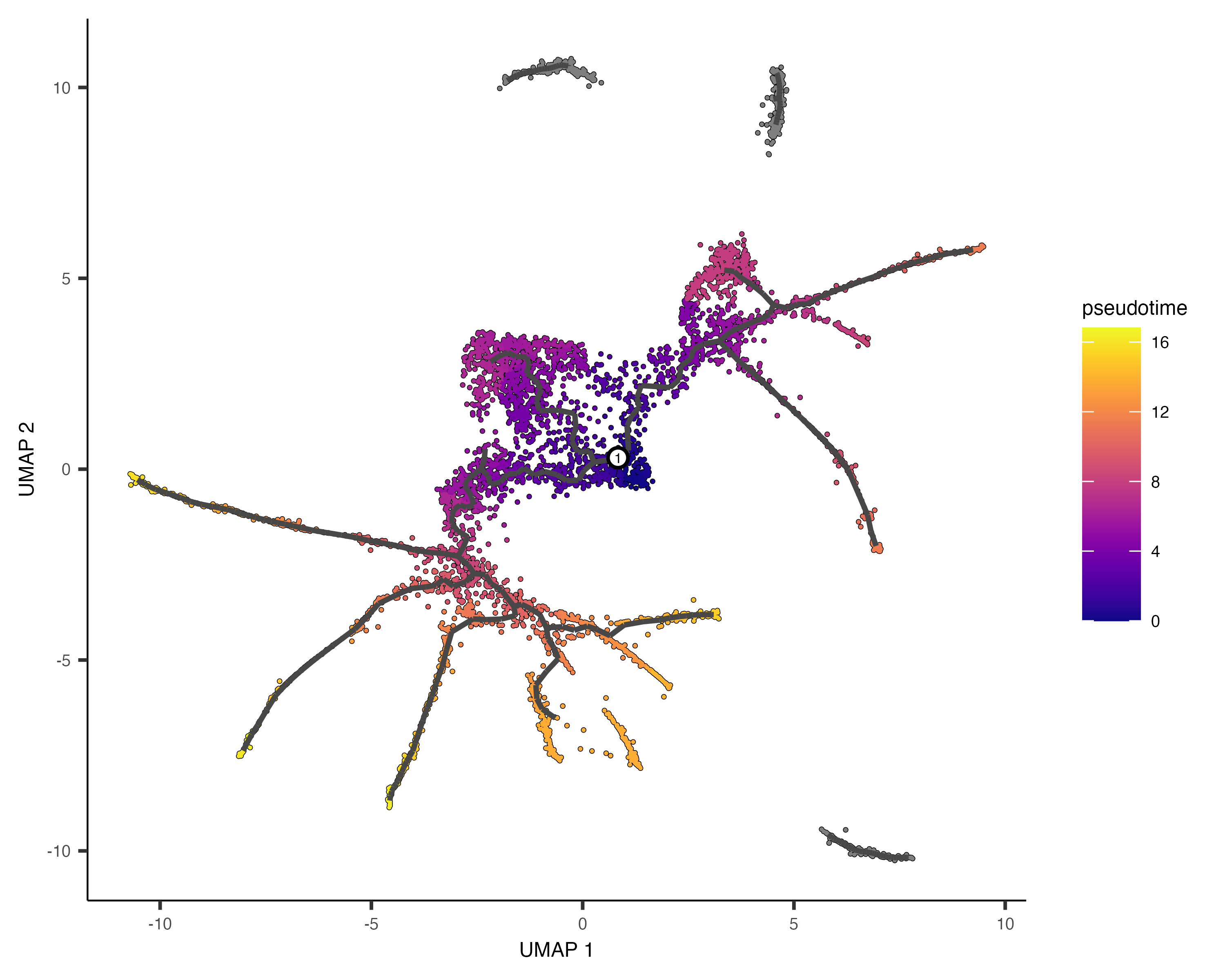

Note that we could easily do this on a per-partition basis by first grouping the cells by partition using the partitions() function. This would result in all cells being assigned a finite pseudotime.

Subset cells by branch

It is often useful to subset cells based on their branch in the trajectory. The function choose_graph_segments allows you to do so interactively.

cds_sub <- choose_graph_segments(cds)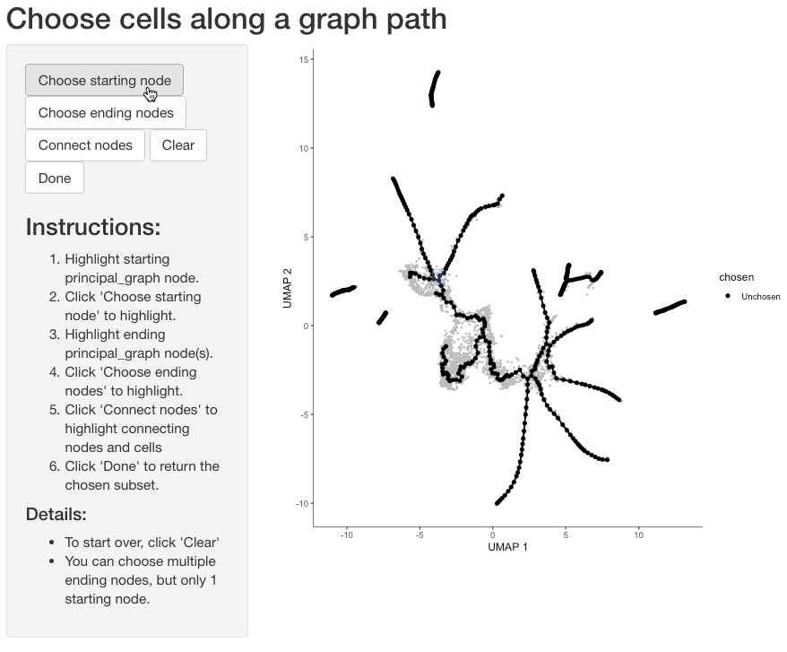

Working with 3D trajectories

cds_3d <- reduce_dimension(cds, max_components = 3)
cds_3d <- cluster_cells(cds_3d)
cds_3d <- learn_graph(cds_3d)
cds_3d <- order_cells(cds_3d, root_pr_nodes=get_earliest_principal_node(cds))

cds_3d_plot_obj <- plot_cells_3d(cds_3d, color_cells_by="partition")