Abstract
Single cell gene expression studies enables one to profile transcriptional regulation in complex biological processes and highly hetergeneous cell populations. These studies facilitate the discovery of genes that identify certain subtypes of cells, or that mark intermediate states during a biological process as well as bifurcate between two alternative cellular fates. In many single cell studies, individual cells are executing through a gene expression program in an unsynchronized manner. In effect, each cell is a snapshot of the transcriptional program under study. The package Monocle provides tools for analyzing single-cell expression experiments. Monocle introduced the strategy of ordering single cells in pseudotime, placing them along a trajectory corresponding to a biological process such as cell differentiation by taking advantage of individual cell's asynchronous progression of those processes. Monocle orders cells by learning an explicit principal graph from the single cell genomics data with advanced machine learning techniques (Reversed Graph Embedding), which robustly and accurately resolves complicated biological processes. Monocle also performs clustering (i.e. using t-SNE and density peaks clustering). Monocle then performs differential gene expression testing, allowing one to identify genes that are differentially expressed between different state, along a biological process as well as alternative cell fates. Monocle is designed for single cell RNA-Seq studies, but can be used with other assays. For more information on the algorithm at the core of Monocle, or to learn more about how to use single cell RNA-Seq to study complex biological processes, explore our publications.
Introduction
The monocle package provides a toolkit for analyzing single cell gene expression experiments. This vignette provides an overview of a single cell RNA-Seq analysis workflow with Monocle. Monocle was originally developed to analyze dynamic biological processes such as cell differentiation, although it also supports other experimental settings.
Monocle 2 includes new and improved algorithms for classifying and counting cells, performing differential expression analysis between subpopulations of cells, and reconstructing cellular trajectories. Monocle 2 has also been re-engineered to work well with very large single-cell RNA-Seq experiments containing tens of thousands of cells or more.
Monocle can help you perform three main types of analysis:
- Clustering, classifying, and counting cells. Single-cell RNA-Seq experiments allow you to discover new (and possibly rare) subtypes of cells. Monocle helps you identify them.
- Constructing single-cell trajectories. In development, disease, and throughout life, cells transition from one state to another. Monocle helps you discover these transitions.
- Differential expression analysis. Characterizing new cell types and states begins with comparing them to other, better understood cells. Monocle includes a sophisticated but easy to use system for differential expression.
Installing Monocle
Required software
Monocle runs in the R statistical
computing environment. You will need R version 3.4 or higher, Bioconductor
version 3.5, and monocle 2.4.0 or higher to have access to the latest features.
To install Bioconductor:
source("http://bioconductor.org/biocLite.R")
biocLite()
Once you've installed Bioconductor, you're ready to install Monocle and all
of its required dependencies:
> biocLite("monocle")
Testing the installation
To ensure that Monocle was installed correctly, start a new R session and type:
library(monocle)
Installing the latest Beta release
The latest stable release of Monocle is available through Bioconductor, and we
recommend you use that. However, you can also install our latest public beta
build through GitHub as show below. Enter the following commands at the R
console:
install.packages("devtools")
devtools::install_github("cole-trapnell-lab/monocle-release@develop")
Sometimes we add features that require you install certain additional packages.
You may see errors when you try the above command. You can install the packages
in the error message by typing (for example):
biocLite(c("DDRTree", "pheatmap"))
Getting help
Questions about Monocle should be posted on our Google Group. Please use monocle.users@gmail.com for private communications that cannot be addressed by the Monocle user community. Please do not email technical questions to Monocle contributors directly.
Recommended analysis protocol
Monocle is a powerful toolkit for analyzing single-cell RNA-seq. You don't need to use all of its features for every analysis, and there are more than one way to do some steps. The workflow is broken up into broad steps. When there's more than one way to do a certain step, we've labeled the options as follows:
| Required | You need to do this. |
| Recommended | Of the ways you could do this, we recommend you try this one first. |
| Alternative | Of the ways you could do this, this way might work better than the one we usually recommend. |
Workflow steps at a glance
Below, you can see snippets of code that highlight the main steps of Monocle. Click on the section headers to jump to the detailed sections describing each one.
Store Data in a CellDataSet Object
The first step in working with Monocle is to load up your data into Monocle's main class,CellDataSet:
pd <- new("AnnotatedDataFrame", data = sample_sheet)
fd <- new("AnnotatedDataFrame", data = gene_annotation)
cds <- newCellDataSet(expr_matrix, phenoData = pd, featureData = fd)
Classify cells with known marker genes
Next, leverage your knowledge of key marker genes to quickly and easily classify your cells by type:cth <- newCellTypeHierarchy()
MYF5_id <- row.names(subset(fData(cds), gene_short_name == "MYF5"))
ANPEP_id <- row.names(subset(fData(cds), gene_short_name == "ANPEP"))
cth <- addCellType(cth, "Myoblast", classify_func =
function(x) { x[MYF5_id,] >= 1 })
cth <- addCellType(cth, "Fibroblast", classify_func =
function(x) { x[MYF5_id,] < 1 & x[ANPEP_id,] > 1 } )
cds <- classifyCells(cds, cth, 0.1)Cluster your cells
You can easily cluster your cells to find new types:cds <- clusterCells(cds)Order cells in pseudotime along a trajectory
Now, put your cells in order by how much progress they've made through whatever process you're studying, such as differentiation, reprogramming, or an immune response.disp_table <- dispersionTable(cds)
ordering_genes <- subset(disp_table, mean_expression >= 0.1)
cds <- setOrderingFilter(cds, ordering_genes)
cds <- reduceDimension(cds)
cds <- orderCells(cds)Perform differential expression analysis
Compare groups of cells in myriad ways to find differentially expressed genes, controlling for batch effects and treatments as you like:diff_test_res <- differentialGeneTest(cds,
fullModelFormulaStr = "~Media")
sig_genes <- subset(diff_test_res, qval < 0.1)Getting Started with Monocle
Monocle takes a matrix of gene expression values as calculated by Cufflinks or another gene expression estimation program. Monocle can work with relative expression values (e.g. FPKM or TPM units) or absolute transcript counts (e.g. from UMI experiments). Monocle also works "out-of-the-box" with the transcript count matrices produced by CellRanger, the software pipeline for analyzing experiments from the 10X Genomics Chromium instrument. Monocle also works well with data from other RNA-Seq workflows such as sci-RNA-Seq and instruments like the Biorad ddSEQ. Although Monocle can be used with raw read counts, these are not directly proportional to expression values unless you normalize them by length, so some Monocle functions could produce nonsense results. If you don't have UMI counts, We recommend you load up FPKM or TPM values instead of raw read counts.The CellDataSet class
Monocle holds single cell expression data in objects of theCellDataSet class. The class is derived from the Bioconductor ExpressionSet class, which provides a common interface familiar to those who have analyzed microarray experiments with Bioconductor. The class requires three input files:
-
exprs, a numeric matrix of expression values, where rows are genes, and columns are cells -
phenoData, anAnnotatedDataFrameobject, where rows are cells, and columns are cell attributes (such as cell type, culture condition, day captured, etc.) -
featureData, anAnnotatedDataFrameobject, where rows are features (e.g. genes), and columns are gene attributes, such as biotype, gc content, etc.
Required dimensions for input files
- have the same number of columns as the
phenoDatahas rows. - have the same number of rows as the
featureDatadata frame has rows.
- row names of the
phenoDataobject should match the column names of the expression matrix. - row names of the
featureDataobject should match row names of the expression matrix. - one of the columns of the
featureDatashould be named "gene_short_name".
You can create a new CellDataSet object as follows:
#do not run
HSMM_expr_matrix <- read.table("fpkm_matrix.txt")
HSMM_sample_sheet <- read.delim("cell_sample_sheet.txt")
HSMM_gene_annotation <- read.delim("gene_annotations.txt")
Once these tables are loaded, you can create the CellDataSet object like this:
pd <- new("AnnotatedDataFrame", data = HSMM_sample_sheet)
fd <- new("AnnotatedDataFrame", data = HSMM_gene_annotation)
HSMM <- newCellDataSet(as.matrix(HSMM_expr_matrix),
    phenoData = pd, featureData = fd)
This will create a CellDataSet object with expression values measured in FPKM, a measure of relative expression reported by Cufflinks. By default, Monocle assumes that your expression data is in units of transcript counts and uses a negative binomial model to test for differential expression in downstream steps. However, if you're using relative expression values such as TPM or FPKM data, see below for how to tell Monocle how to model it in downstream steps.
Don't normalize data yourself
CellDataSet.
You should also not try to convert the UMI counts to relative abundances (by converting it to FPKM/TPM data).
You should not use relative2abs() as discussed below in the section on Converting TPM to mRNA Counts. Monocle will do all needed normalization steps internally.
Normalizing it yourself risks breaking some of Monocle's key steps.
Importing & exporting data with other packages
This function will be available after the next BioConductor release, 10/31. Monocle is able to convert Seurat objects from the package "Seurat" and SCESets from the package
"scater" into CellDataSet objects that Monocle can use.
It's also worth noting that the function will also work with SCESets from "Scran".
To convert from either a Seurat object or a SCESet
to a CellDataSet, execute the function importCDS() as shown:
# Where 'data_to_be_imported' can either be a Seurat object
# or an SCESet.

importCDS(data_to_be_imported)

# We can set the parameter 'import_all' to TRUE if we'd like to
# import all the slots from our Seurat object or SCESet.
# (Default is FALSE or only keep minimal dataset)

importCDS(data_to_be_imported, import_all = TRUE)
Monocle can also export data from CellDataSets to the "Seurat" and "scater" packages through the
function exportCDS():
lung <- load_lung()

# To convert to Seurat object
lung_seurat <- exportCDS(lung, 'Seurat')

# To convert to SCESet
lung_SCESet <- exportCDS(lung, 'Scater')
Choosing a distribution for your data Required
Monocle works well with both relative expression data and count-based measures (e.g. UMIs).
In general, it works best with transcript count data, especially UMI data.
Whatever your data type, it is critical that specify the appropriate distribution for it.
FPKM/TPM values are generally log-normally distributed, while UMIs or read counts are better modeled with the negative binomial.
To work with count data, specify the negative binomial distribution as the expressionFamily argument to newCellDataSet:
#Do not run
HSMM <- newCellDataSet(count_matrix,
                phenoData = pd,
                featureData = fd,
                expressionFamily=negbinomial.size())
There are several allowed values for expressionFamily, which expects a "family function" from the VGAM package:
| Family function | Data type | Notes |
|---|---|---|
negbinomial.size() |
UMIs, Transcript counts from experiments with spike-ins or relative2abs(), raw read counts |
Negative binomial distribution with fixed variance (which is automatically calculated by Monocle). Recommended for most users. |
negbinomial() |
UMIs, Transcript counts from experiments with spike-ins or relative2abs, raw read counts |
Slightly more accurate than negbinomial.size(), but much, much slower. Not recommended except for very small datasets. |
tobit() |
FPKM, TPM | Tobits are truncated normal distributions. Using tobit() will tell Monocle to log-transform your data where appropriate. Do not transform it yourself. |
gaussianff() |
log-transformed FPKM/TPMs, Ct values from single-cell qPCR | If you want to use Monocle on data you have already transformed to be normally distributed, you can use this function, though some Monocle features may not work well. |
Use the right distribution!
relative2abs().
This often leads to much more accurate results than using tobit(). See the section on Converting TPM to mRNA Counts for details.
Working with large data sets Recommended
Some single-cell RNA-Seq experiments report measurements from tens of thousands of cells or more. As instrumentation improves and costs drop, experiments will become ever larger and more complex, with many conditions, controls, and replicates. A matrix of expression data with 50,000 cells and a measurement for each of the 25,000+ genes in the human genome can take up a lot of memory. However, because current protocols typically don't capture all or even most of the mRNA molecules in each cell, many of the entries of expression matrices are zero. Using sparse matrices can help you work with huge datasets on a typical computer. We generally recommend the use of sparseMatrices for most users, as it speeds up many computations even for more modestly sized datasets.
To work with your data in a sparse format, simply provide it to Monocle as a sparse matrix from the Matrix package:
HSMM <- newCellDataSet(as(umi_matrix, "sparseMatrix"),
                phenoData = pd,
                featureData = fd,
                lowerDetectionLimit = 0.5,
                expressionFamily = negbinomial.size())
Don't accidentally convert to a dense expression matrix
as.matrix(), because that may exceed your available memeory.
cellrangerRkit, you can use it to load your data and then pass that to Monocle as follows:
cellranger_pipestance_path <- "/path/to/your/pipeline/output/directory"
gbm <- load_cellranger_matrix(cellranger_pipestance_path)

fd <- fData(gbm)

# The number 2 is picked arbitrarily in the line below.
# Where "2" is placed you should place the column number that corresponds to your
# featureData's gene short names.

colnames(fd)[2] <- "gene_short_name"

gbm_cds <- newCellDataSet(exprs(gbm),
                  phenoData = new("AnnotatedDataFrame", data = pData(gbm)),
                  featureData = new("AnnotatedDataFrame", data = fd),
                  lowerDetectionLimit = 0.5,
expressionFamily = negbinomial.size())Matrix package.
Other sparse matrix packages, such as slam or SparseM are not supported.
Converting TPM/FPKM values into mRNA counts Alternative
If you performed your single-cell RNA-Seq experiment using spike-in standards, you can convert these measurements into mRNAs per cell (RPC).
RPC values are often easier to analyze than FPKM or TPM values, because have better statistical tools to model them.
In fact, it's possible to convert FPKM or TPM values to RPC values even if there were no spike-in standards included in the experiment.
Monocle 2 includes an algorithm called Census which performs this conversion [8].
You can convert to RPC values before creating your CellDataSet object using the relative2abs() function, as follows:
pd <- new("AnnotatedDataFrame", data = HSMM_sample_sheet)
fd <- new("AnnotatedDataFrame", data = HSMM_gene_annotation)

# First create a CellDataSet from the relative expression levels
HSMM <- newCellDataSet(as.matrix(HSMM_expr_matrix),
                phenoData = pd,
                featureData = fd,
                lowerDetectionLimit = 0.1,
                expressionFamily = tobit(Lower = 0.1))

# Next, use it to estimate RNA counts
rpc_matrix <- relative2abs(HSMM, method = "num_genes")

# Now, make a new CellDataSet using the RNA counts
HSMM <- newCellDataSet(as(as.matrix(rpc_matrix), "sparseMatrix"),
                phenoData = pd,
                featureData = fd,
                lowerDetectionLimit = 0.5,
                expressionFamily = negbinomial.size())
TPM/FPKM data and mRNA count data use different arguments to newCellDataSet()
lowerDetectionLimit to reflect the new scale of expression.
Importantly, we have also set the expressionFamily to negbinomial(), which tells Monocle to use the negative binomial distribution in certain downstream statistical tests.
Failing to change these two options can create problems later on, so make sure not to forget them when using Census counts.
Estimate size factors and dispersions Required
Finally, we'll also call two functions that pre-calculate some information about the data. Size factors help us normalize for differences in mRNA recovered across cells, and "dispersion" values will help us perform differential expression analysis later.
Requirements fot estimateSizeFactors and estimateDispersions
estimateSizeFactors() and estimateDispersions() will only work, and are only needed, if you are working with
a CellDataSet with a negbinomial() or negbinomial.size() expression family.
HSMM <- estimateSizeFactors(HSMM)
HSMM <- estimateDispersions(HSMM)
We're now ready to start using the HSMM object in our analysis.
Filtering low-quality cells Recommended
The first step in any single-cell RNA-Seq analysis is identifying poor-quality libraries from further analysis. Most single-cell workflows will include at least some libraries made from dead cells or empty wells in a plate. It's also crucial to remove doublets: libraries that were made from two or more cells accidentally. These cells can disrupt downstream steps like pseudotime ordering or clustering. This section walks through typical quality control steps that should be performed as part of all analyses with Monocle.
It is often convenient to know how many express a particular gene, or how many genes are expressed by a given cell. Monocle provides a simple function to compute those statistics:
HSMM <- detectGenes(HSMM, min_expr = 0.1)
print(head(fData(HSMM)))
| gene_short_name | biotype | num_cells_expressed | use_for_ordering | |
|---|---|---|---|---|
| ENSG00000000003.10 | TSPAN6 | protein_coding | 184 | FALSE |
| ENSG00000000005.5 | TNMD | protein_coding | 0 | FALSE |
| ENSG00000000419.8 | DPM1 | protein_coding | 211 | FALSE |
| ENSG00000000457.8 | SCYL3 | protein_coding | 18 | FALSE |
| ENSG00000000460.12 | C1orf112 | protein_coding | 47 | TRUE |
| ENSG00000000938.8 | FGR | protein_coding | 0 | FALSE |
HSMM <- detectGenes(HSMM, min_expr = 0.1)
print(head(fData(HSMM)))
expressed_genes <- row.names(subset(fData(HSMM),
    num_cells_expressed >= 10))
The vector expressed_genes now holds the identifiers for genes expressed in at least 50 cells of the data set.
We will use this list later when we put the cells in order of biological progress.
It is also sometimes convenient to exclude genes expressed in few if any cells from the CellDataSet object so as not to waste CPU time analyzing them for differential expression.
Let's start trying to remove unwanted, poor quality libraries from the CellDataSet. Your single cell RNA-Seq protocol may have given you the opportunity to image individual cells after capture but prior to lysis. This image data allows you to score your cells, confirming that none of your libraries were made from empty wells or wells with excess cell debris. With some protocols and instruments, you may get more than one cell captured instead just a single cell. You should exclude libraries that you believe did not come from a single cell, if possible. Empty well or debris well libraries can be especially problematic for Monocle. It's also a good idea to check that each cell's RNA-seq library was sequenced to an acceptible degree.
While there is no widely accepted minimum level for what constitutes seequencing "deeply enough", use your judgement: a cell sequenced with only a few thousand reads is unlikely to yield meaningful measurements.
CellDataSet objects provide a convenient place to store per-cell scoring data: the phenoData slot.
Simply include scoring attributes as columns in the data frome you used to create your CellDataSet container.
You can then easily filter out cells that don't pass quality control.
You might also filter cells based on metrics from high throughput sequencing quality assessment packages such as FastQC.
Such tools can often identify RNA-Seq libraries made from heavily degraded RNA, or where the library contains an abnormally large amount of ribosomal, mitochondrial, or other RNA type that you might not be interested in.
The HSMM dataset included with this package has scoring columns built in:
print(head(pData(HSMM)))
| Library | Well | Hours | Media | Mapped.Fragments | Pseudotime | State | Size_Factor | num_genes_expressed | |
|---|---|---|---|---|---|---|---|---|---|
| T0_CT_A01 | SCC10013_A01 | A01 | 0 | GM | 1958074 | 23.916673 | 1 | 1.392811 | 6850 |
| T0_CT_A03 | SCC10013_A03 | A03 | 0 | GM | 1930722 | 9.022265 | 1 | 1.311607 | 6947 |
| T0_CT_A05 | SCC10013_A05 | A05 | 0 | GM | 1452623 | 7.546608 | 1 | 1.218922 | 7019 |
| T0_CT_A06 | SCC10013_A06 | A06 | 0 | GM | 2566325 | 21.463948 | 1 | 1.013981 | 5560 |
| T0_CT_A07 | SCC10013_A07 | A07 | 0 | GM | 2383438 | 11.299806 | 1 | 1.085580 | 5998 |
| T0_CT_A08 | SCC10013_A08 | A08 | 0 | GM | 1472238 | 67.436042 | 2 | 1.099878 | 6055 |
valid_cells <- row.names(subset(pData(HSMM),
            Cells.in.Well == 1 &
            Control == FALSE &
            Clump == FALSE &
            Debris == FALSE &
            Mapped.Fragments > 1000000))
HSMM <- HSMM[,valid_cells]
If you are using RPC values to measure expression, as we are in this vignette, it's also good to look at the distribution of mRNA totals across the cells:
pData(HSMM)$Total_mRNAs <- Matrix::colSums(exprs(HSMM))

HSMM <- HSMM[,pData(HSMM)$Total_mRNAs < 1e6]

upper_bound <- 10^(mean(log10(pData(HSMM)$Total_mRNAs)) +
            2*sd(log10(pData(HSMM)$Total_mRNAs)))
lower_bound <- 10^(mean(log10(pData(HSMM)$Total_mRNAs)) -
            2*sd(log10(pData(HSMM)$Total_mRNAs)))

qplot(Total_mRNAs, data = pData(HSMM), color = Hours, geom =
"density") +
geom_vline(xintercept = lower_bound) +
geom_vline(xintercept = upper_bound)
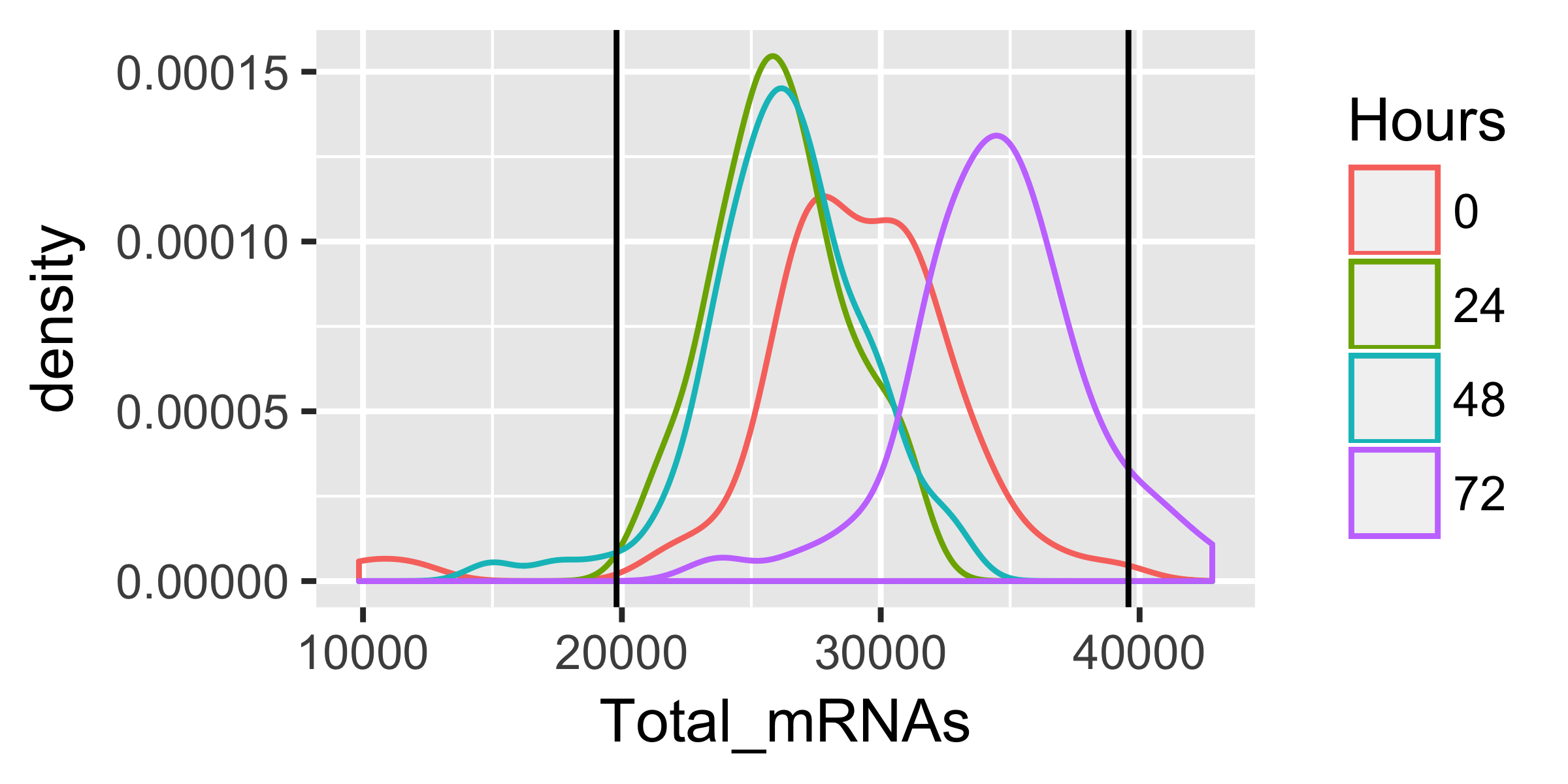
HSMM <- HSMM[,pData(HSMM)$Total_mRNAs > lower_bound &
      pData(HSMM)$Total_mRNAs < upper_bound]
HSMM <- detectGenes(HSMM, min_expr = 0.1)
CellDataSet follow a distribution that is roughly lognormal:
# Log-transform each value in the expression matrix.
L <- log(exprs(HSMM[expressed_genes,]))

# Standardize each gene, so that they are all on the same scale,
# Then melt the data with plyr so we can plot it easily
melted_dens_df <- melt(Matrix::t(scale(Matrix::t(L))))

# Plot the distribution of the standardized gene expression values.
qplot(value, geom = "density", data = melted_dens_df) +
stat_function(fun = dnorm, size = 0.5, color = 'red') +
xlab("Standardized log(FPKM)") +
ylab("Density")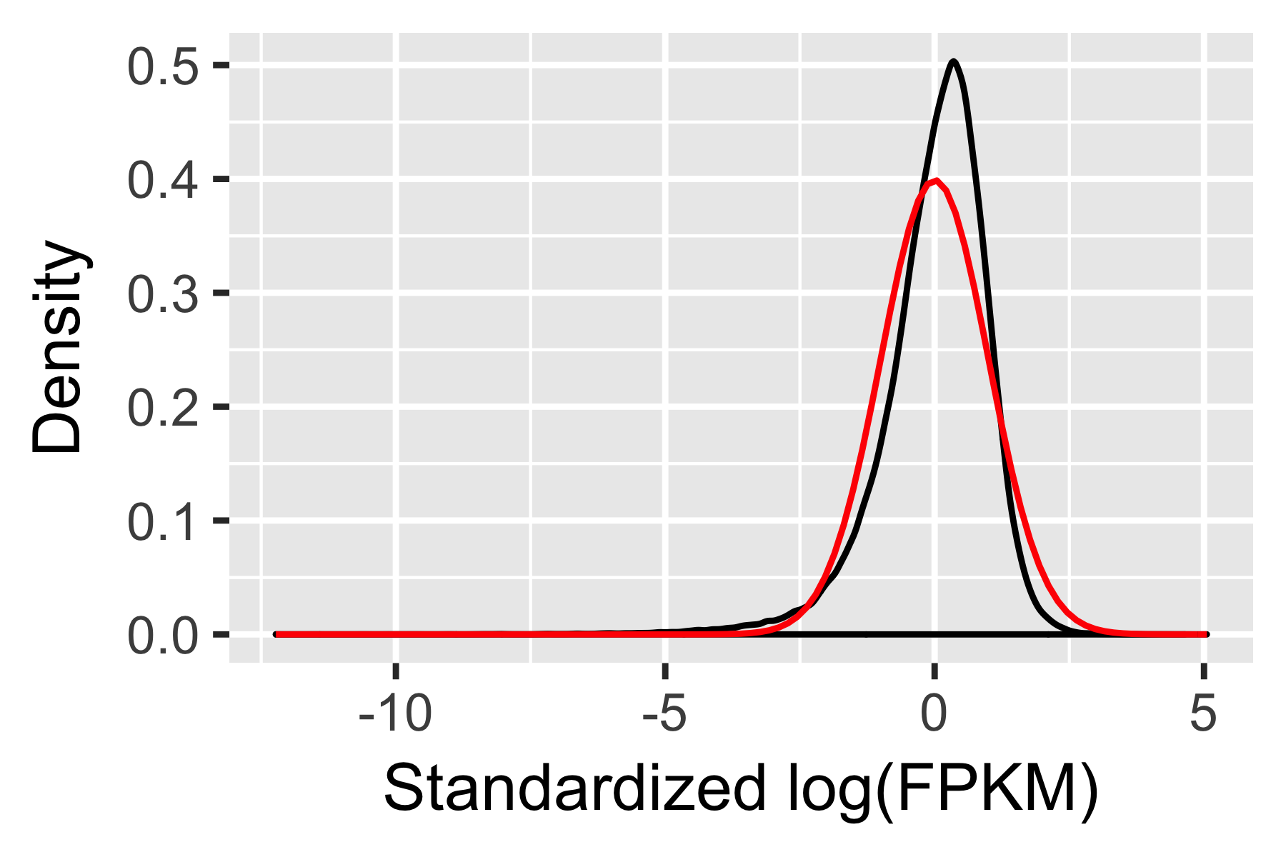
Classifying and Counting Cells
Single cell experiments are often performed on complex mixtures of multiple cell types. Dissociated tissue samples might contain two, three, or even many different cells types. In such cases, it's often nice to classify cells based on type using known markers. In the myoblast experiment, the culture contains fibroblasts that came from the original muscle biopsy used to establish the primary cell culture. Myoblasts express some key genes that fibroblasts don't. Selecting only the genes that express, for example, sufficiently high levels of MYF5 excludes the fibroblasts. Likewise, fibroblasts express high levels of ANPEP (CD13), while myoblasts tend to express few if any transcripts of this gene.
Classifying cells by type Recommended
Monocle provides a simple system for tagging cells based on the expression of marker genes of your choosing. You simply provide a set of functions that Monocle can use to annotate each cell. For example, you could provide a function for each of several cell types. These functions accept as input the expression data for each cell, and return TRUE to tell Monocle that a cell meets the criteria defined by the function. So you could have one function that returns TRUE for cells that express myoblast-specific genes, another function for fibroblast-specific genes, etc. Here's an example of such a set of "gating" functions:
MYF5_id <- row.names(subset(fData(HSMM), gene_short_name == "MYF5"))
ANPEP_id <- row.names(subset(fData(HSMM),
    gene_short_name == "ANPEP"))

cth <- newCellTypeHierarchy()
cth <- addCellType(cth, "Myoblast", classify_func =
    function(x) { x[MYF5_id,] >= 1 })
cth <- addCellType(cth, "Fibroblast", classify_func = function(x)
 { x[MYF5_id,] < 1 & x[ANPEP_id,] > 1 })
CellTypeHierarchy, that Monocle uses to classify the cells.
You first initialize a new CellTypeHierarchy object, then register your gating functions within it.
Once the data structure is set up, you can use it to classify all the cells in the experiment:
HSMM <- classifyCells(HSMM, cth, 0.1)
The function classifyCells applies each gating function to each cell, classifies the cells according to the gating functions, and returns the CellDataSet with a new column, CellType in its pData table.
We can now count how many cells of each type there are in the experiment.
table(pData(HSMM)$CellType)
| Fibroblast | Myoblast | Unknown |
|---|---|---|
| 56 | 85 | 121 |
pie <- ggplot(pData(HSMM),
aes(x = factor(1), fill = factor(CellType))) + geom_bar(width = 1)
pie + coord_polar(theta = "y") +
theme(axis.title.x = element_blank(), axis.title.y = element_blank())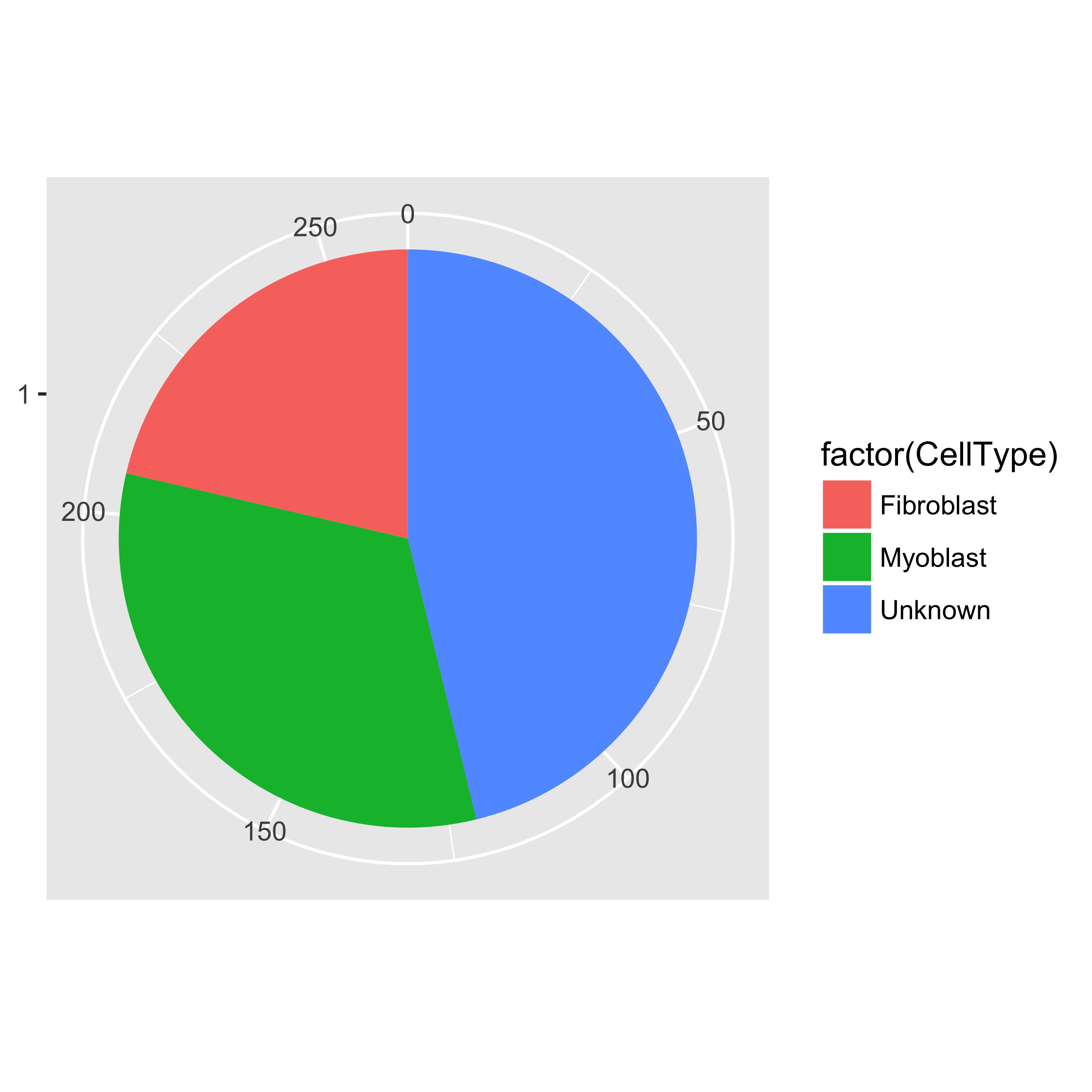
Clustering cells without marker genes Alternative
Monocle provides an algorithm you can use to impute the types of the "Unknown" cells.
This algorithm, implemented in the function clusterCells, groups cells together according to global expression profile.
That way, if your cell expresses lots of genes specific to myoblasts, but just happens to lack MYF5, we can still recognize it as a myoblast.
clusterCells can be used in an unsupervised manner, as well as in a ``semi-supervised'' mode, which allows to assist the algorithm with some expert knowledge.
Let's look at the unsupervised mode first.
The first step is to decide which genes to use in clustering the cells. We could use all genes, but we'd be including a lot of genes that are not expressed at a high enough level to provide a meaningful signal. Including them would just add noise to the system. We can filter genes based on average expression level, and we can additionally select genes that are unusually variable across cells. These genes tend to be highly informative about cell state.
disp_table <- dispersionTable(HSMM)
unsup_clustering_genes <- subset(disp_table, mean_expression >= 0.1)
HSMM <- setOrderingFilter(HSMM, unsup_clustering_genes$gene_id)
plot_ordering_genes(HSMM)
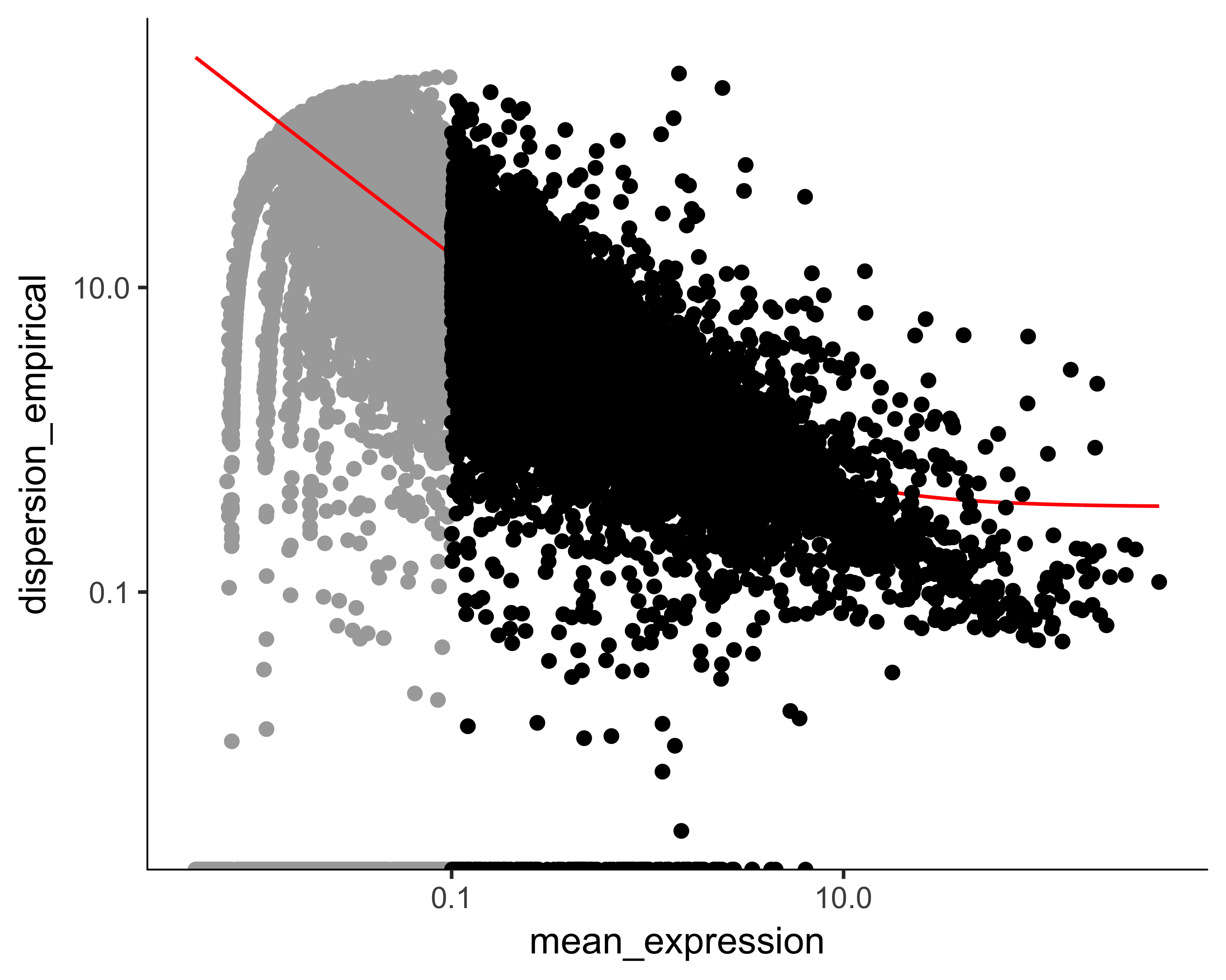
The setOrderingFilter function marks genes that will be used for clustering in subsequent calls to clusterCells, although we will be able to provide other lists of genes if we want.
The plot_ordering_genes function shows how variability (dispersion) in a gene's expression depends on the average expression across cells.
The red line shows Monocle's expectation of the dispersion based on this relationship.
The genes we marked for use in clustering are shown as black dots, while the others are shown as grey dots.
# HSMM@auxClusteringData[["tSNE"]]$variance_explained <- NULL
plot_pc_variance_explained(HSMM, return_all = F) # norm_method='log'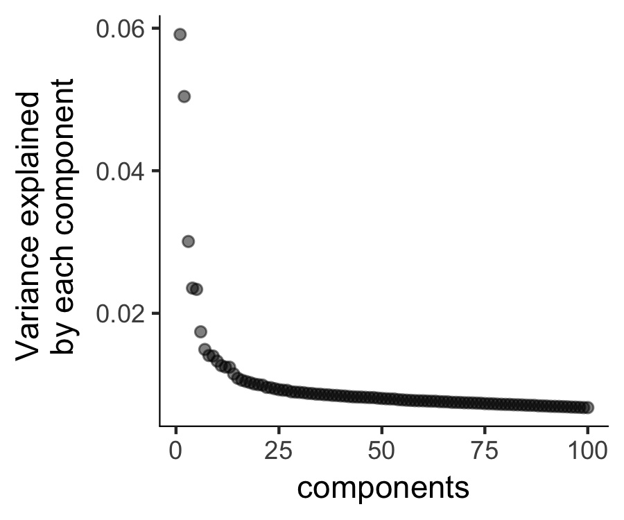
HSMM <- reduceDimension(HSMM, max_components = 2, num_dim = 6,
reduction_method = 'tSNE', verbose = T)
HSMM <- clusterCells(HSMM, num_clusters = 2)
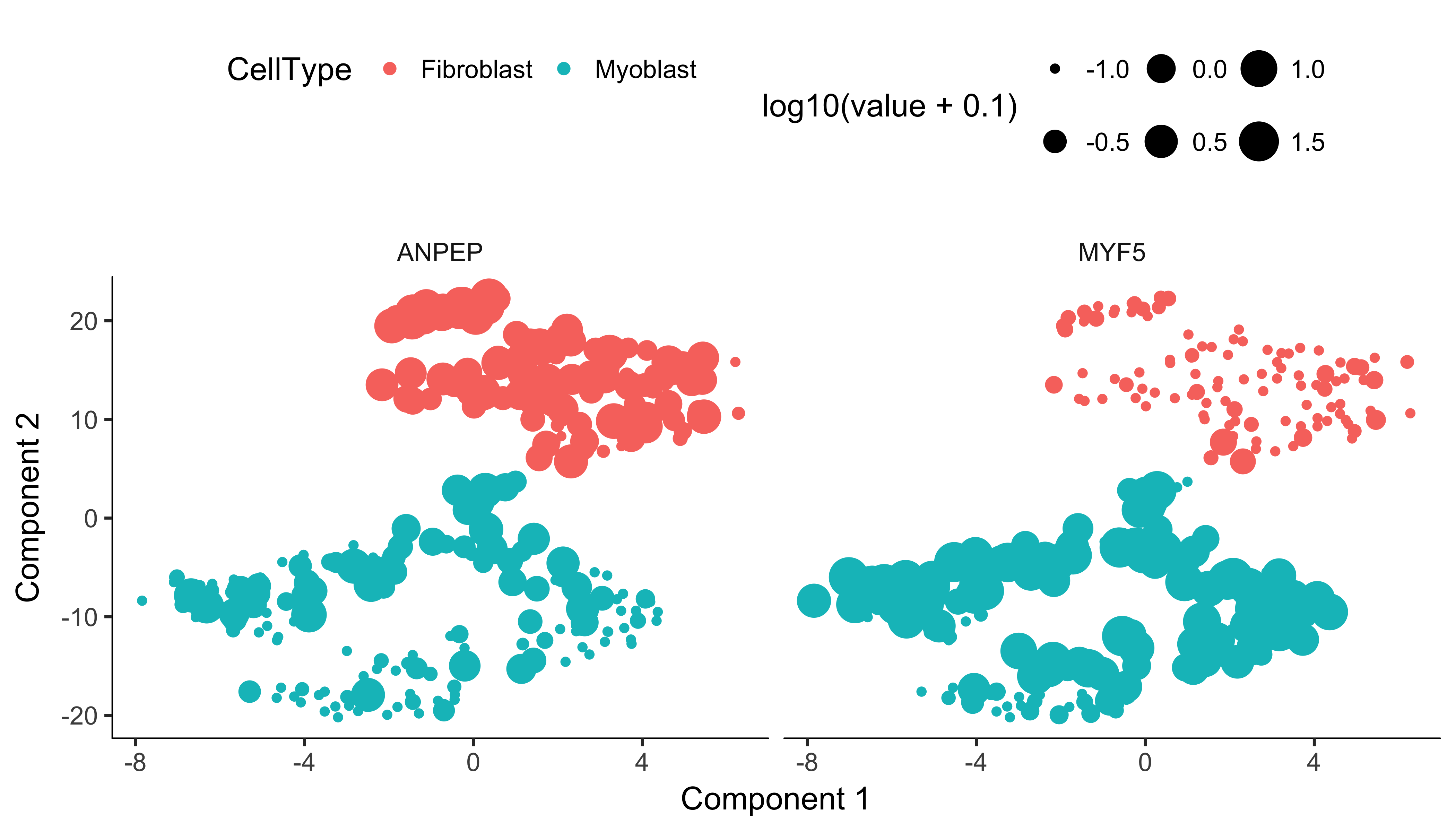
plot_cell_clusters(HSMM, 1, 2, color = "CellType",
markers = c("MYF5", "ANPEP"))Monocle uses t-SNE [3] to cluster cells, using an approach that's very similar to and inspired by Rahul Satija's excellent Seurat package , which itself was inspired by viSNE from Dana Pe'er's lab.
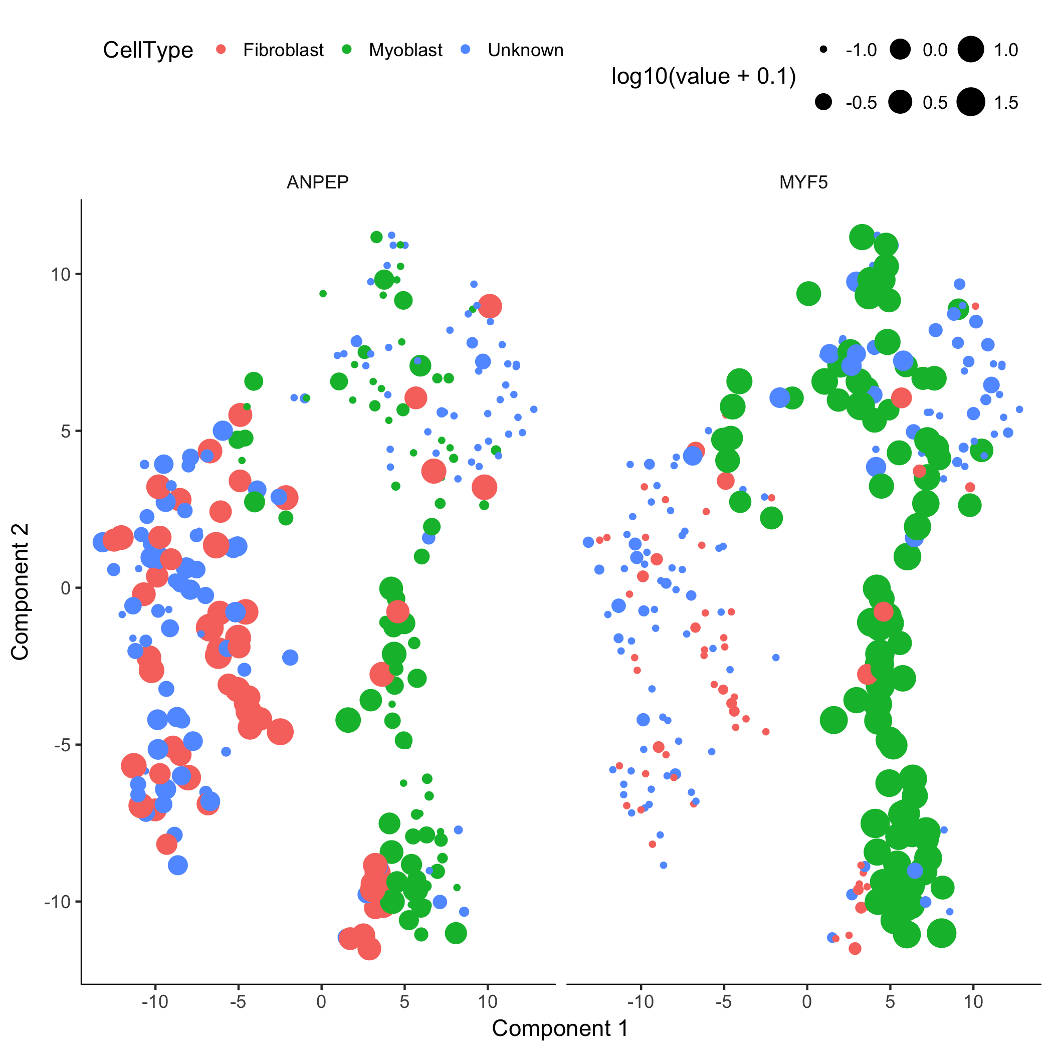
The cells tagged as myoblasts by our gating functions are marked in green, while the fibroblasts are tagged in red. The cells that don't express either marker are blue. In many experiments, cells of different types are clearly separate from one another. Unfortunately, in this experiment, the cells don't simply cluster by type - there's not a clear space between the green cells and the red cells. This isn't all that surprising, because myoblasts and contaminating interstitial fibroblasts express many of the same genes in these culture conditions, and there are multiple culture conditions in the experiment. That is, there are other sources of variation in the experiment that might be driving the clustering. One source of variation in the experiment stems from the experimental design. To initiate myoblast differentiation, we switch media from a high-mitogen growth medium (GM) to a low-mitogen differentiation medium (DM). Perhaps the cells are clustering based on the media they're cultured in?
plot_cell_clusters(HSMM, 1, 2, color = "Media")
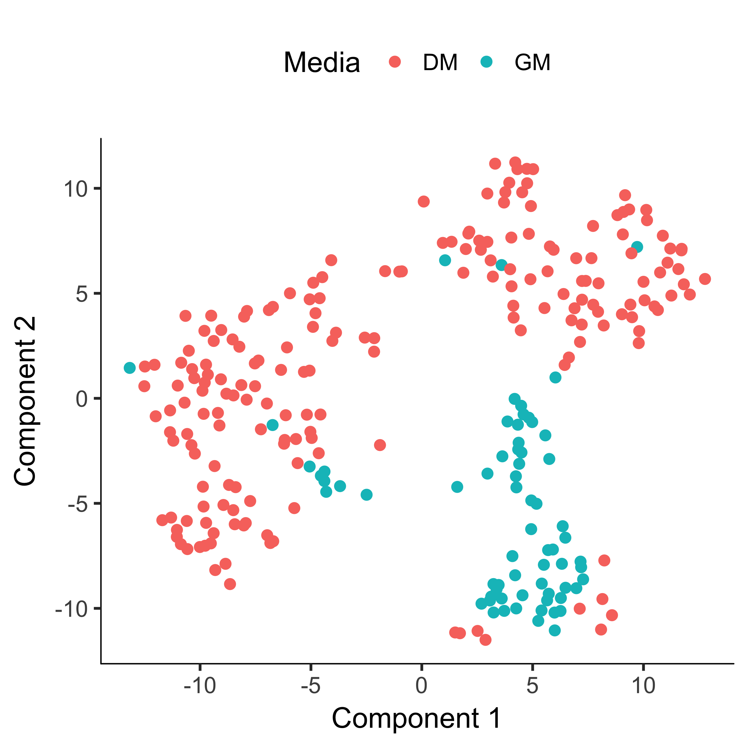
Monocle allows us to subtract the effects of "uninteresting" sources of variation to reduce their impact on the clustering.
You can do this with the residualModelFormulaStr argument to clusterCells and several other Monocle functions.
This argument accepts an R model formula string specifying the effects you want to subtract prior to clustering.
HSMM <- reduceDimension(HSMM, max_components = 2, num_dim = 2,
reduction_method = 'tSNE',
residualModelFormulaStr = "~Media + num_genes_expressed",
verbose = T)
HSMM <- clusterCells(HSMM, num_clusters = 2)
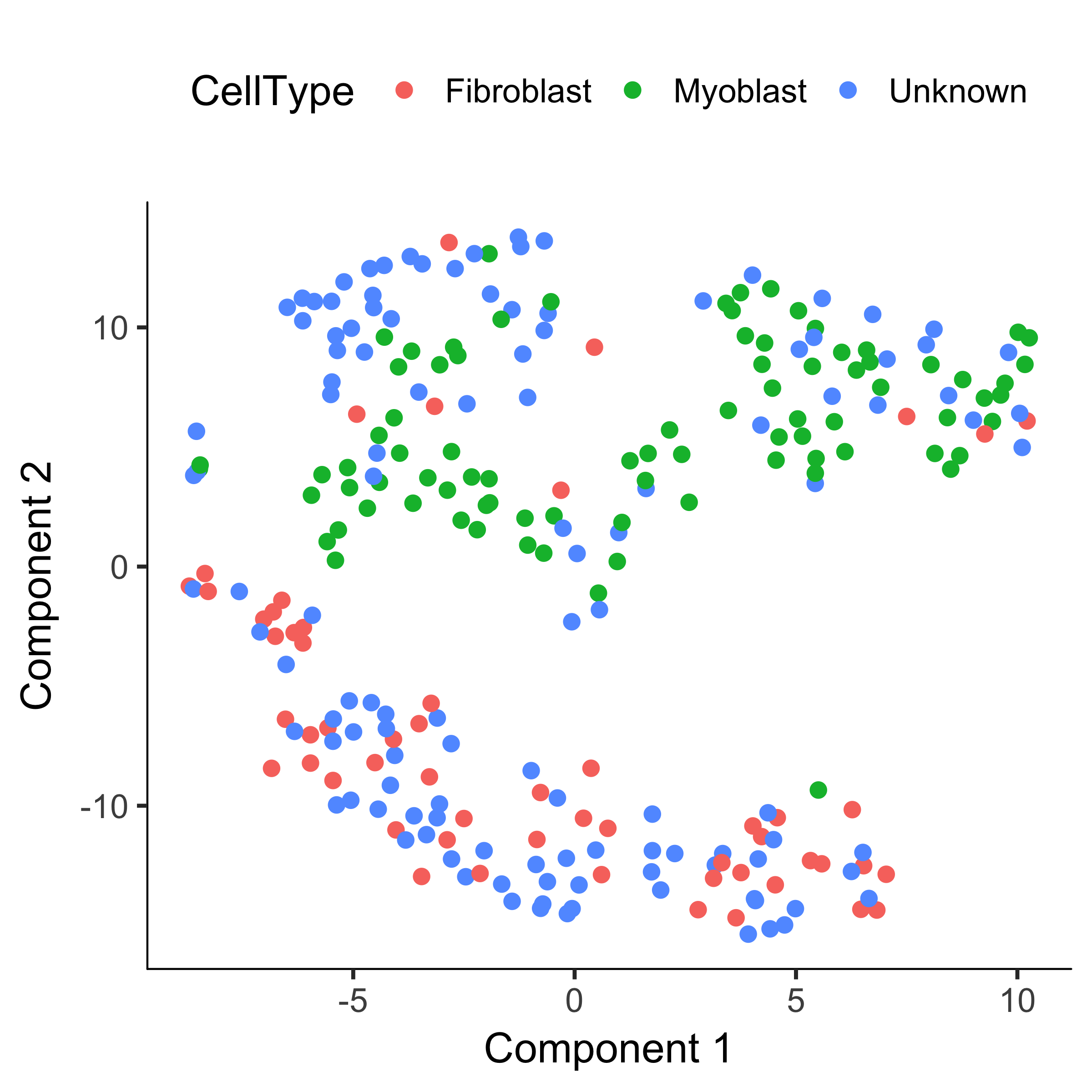
plot_cell_clusters(HSMM, 1, 2, color = "CellType")
HSMM <- clusterCells(HSMM, num_clusters = 2)
plot_cell_clusters(HSMM, 1, 2, color = "Cluster") +
    facet_wrap(~CellType)
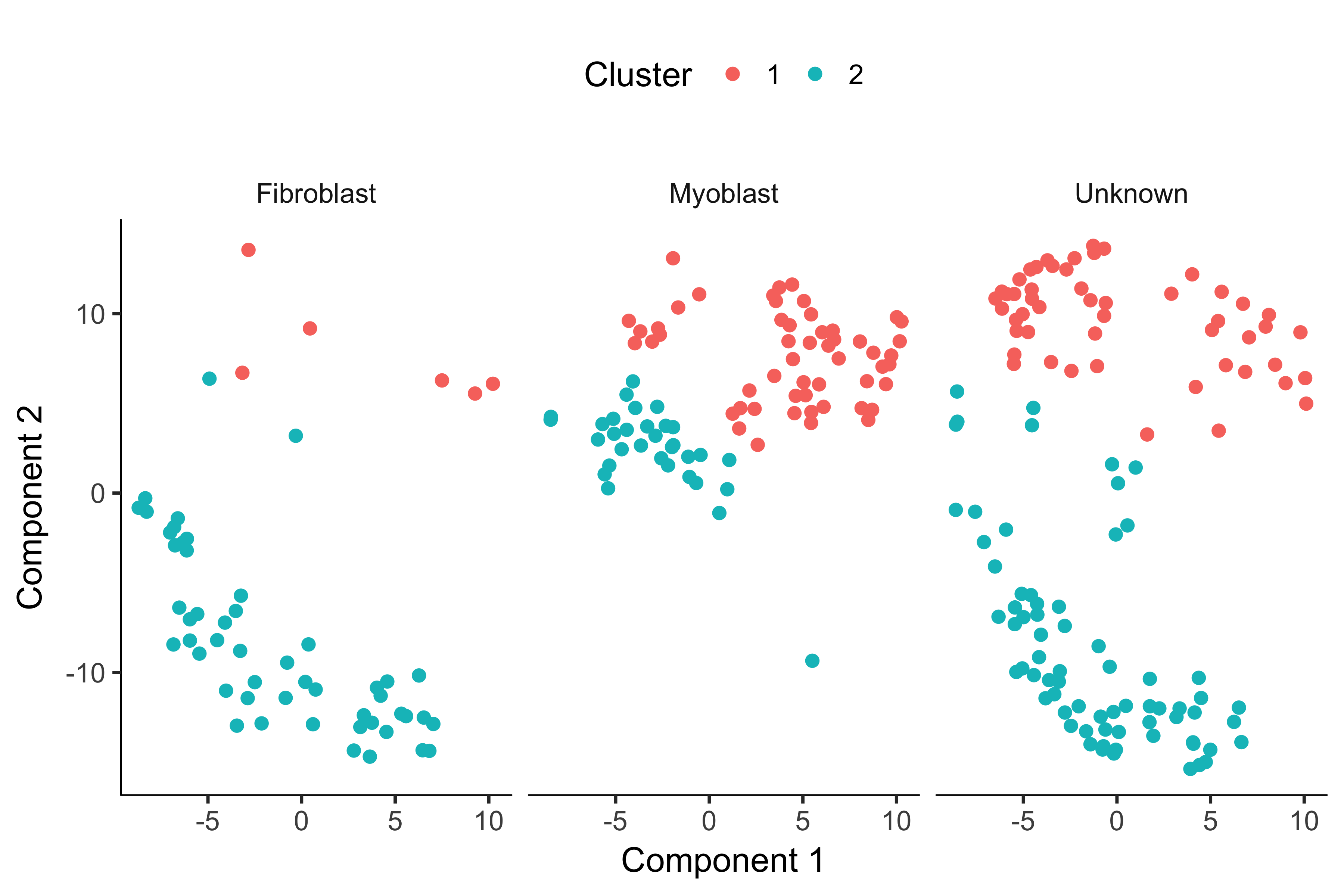
Now, most of the myoblasts are in one cluster, most of the fibroblasts are in the other, and the unknowns are spread across both.
However, we still see some cells of both types in each cluster.
This could be due to lack of specificity in our marker genes and our CellTypeHierarchy functions, but it could also be due to suboptimal clustering.
To help rule out the latter, let's try running clusterCells in its semi-supervised mode.
Clustering cells using marker genes Recommended
First, we'll select a different set of genes to use for clustering the cells. Before we just picked genes that were highly expressed and highly variable. Now, we'll pick genes that co-vary with our markers. In a sense, we'll be building a large list of genes to use as markers, so that even if a cell doesn't have MYF5, it might be recognizable as a myoblast based on other genes.
marker_diff <- markerDiffTable(HSMM[expressed_genes,],
            cth,
            residualModelFormulaStr = "~Media + num_genes_expressed",
            cores = 1)
The function markerDiffTable takes a CellDataSet and a CellTypeHierarchy and classifies all the cells into types according to your provided functions.
It then removes all the "Unknown" and "Ambiguous" functions before identifying genes that are differentially expressed between the types.
Again, you can provide a residual model of effects to exclude from this test.
The function then returns a data frame of test results, and you can use this to pick the genes you want to use for clustering.
Often it's best to pick the top 10 or 20 genes that are most specific for each cell type.
This ensures that the clustering genes aren't dominated by markers for one cell type.
You generally want a balanced panel of markers for each type if possible.
Monocle provides a handy function for ranking genes by how restricted their expression is for each type.
candidate_clustering_genes <-
    row.names(subset(marker_diff, qval < 0.01))
marker_spec <-
  calculateMarkerSpecificity(HSMM[candidate_clustering_genes,], cth)
head(selectTopMarkers(marker_spec, 3))
The last line above shows the top three marker genes for myoblasts and fibroblasts. The "specificity" score is calculated using the metric described in Cabili et al [13] and can range from zero to one. The closer it is to one, the more restricted it is to the cell type in question. You can use this feature to define new markers for known cell types, or pick out genes you can use in purifying newly discovered cell types. This can be highly valuable for downstream follow up experiments.
To cluster the cells, we'll choose the top 500 markers for each of these cell types:semisup_clustering_genes <- unique(selectTopMarkers(marker_spec, 500)$gene_id)
HSMM <- setOrderingFilter(HSMM, semisup_clustering_genes)
plot_ordering_genes(HSMM)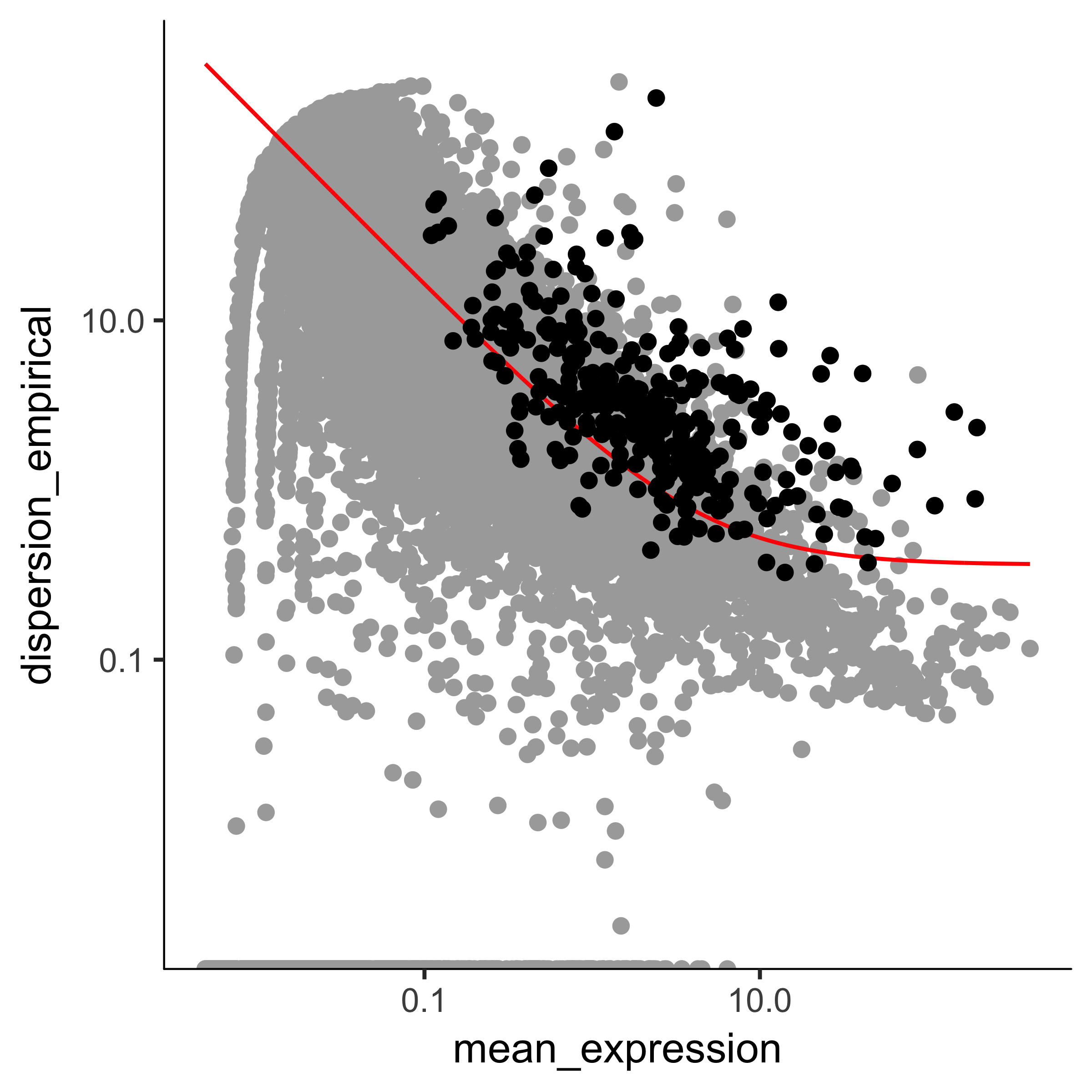
Note that we've got smaller set of genes, and some of them are not
especially highly expressed or variable across the experiment. However, they are
great for distinguishing cells that express MYF5 from those that have
ANPEP. We've already marked them for use in clustering, but even if we
hadn't, we could still use them by providing them directly to
clusterCells.
plot_pc_variance_explained(HSMM, return_all = F)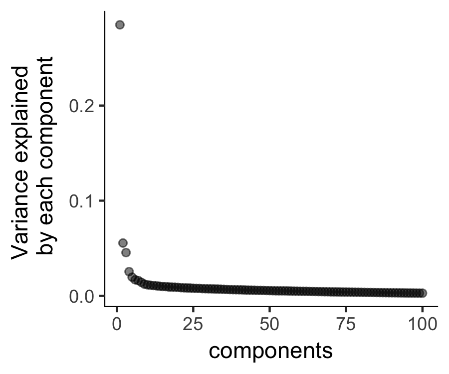
HSMM <- reduceDimension(HSMM, max_components = 2, num_dim = 3,
  norm_method = 'log',
  reduction_method = 'tSNE',
  residualModelFormulaStr = "~Media + num_genes_expressed",
  verbose = T)
HSMM <- clusterCells(HSMM, num_clusters = 2)
plot_cell_clusters(HSMM, 1, 2, color = "CellType")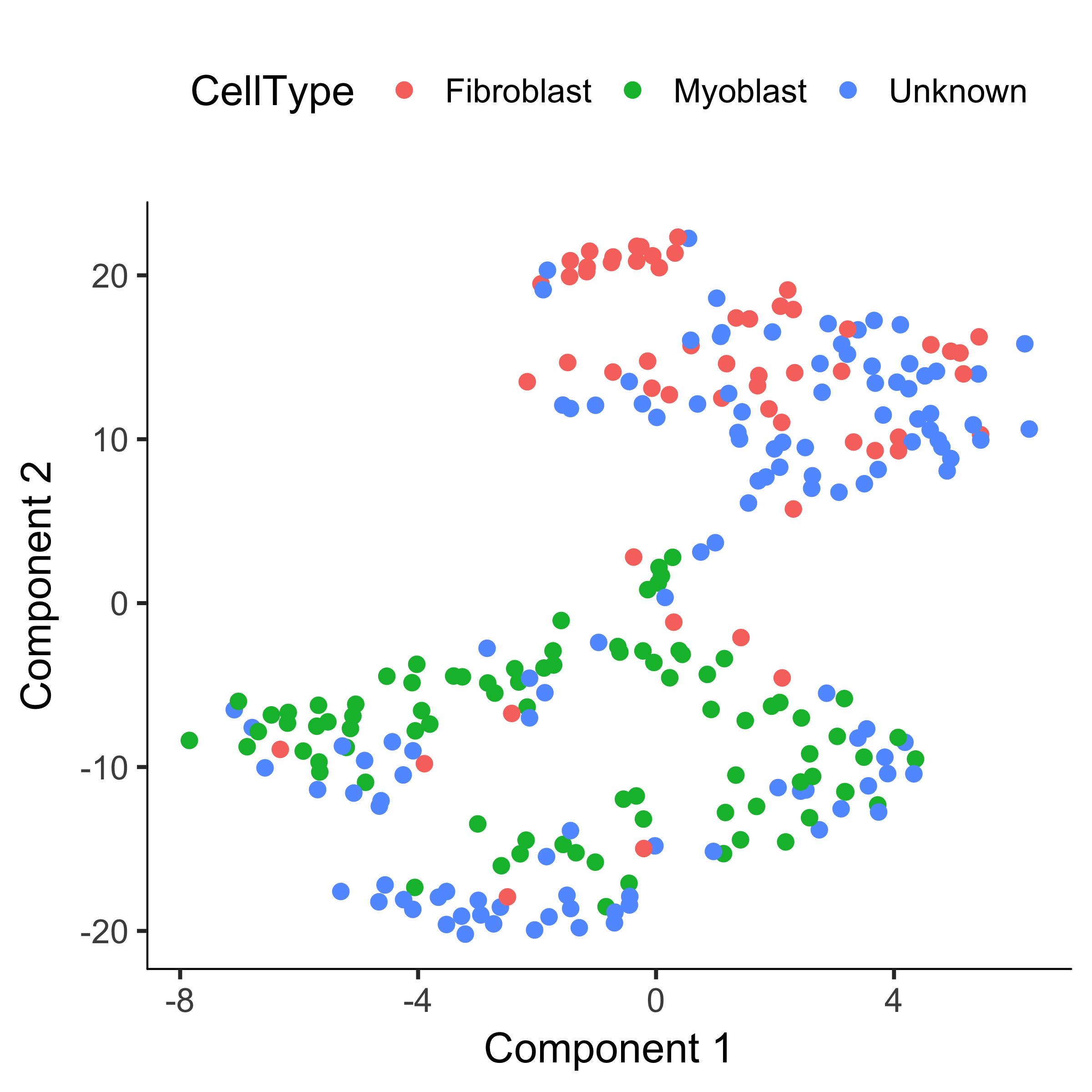
Imputing cell type Alternative
Note that we've reduced the number of "contaminating" fibroblasts in the myoblast cluster, and vice versa.
But what about the "Unknown" cells? If you provide clusterCells with a the CellTypeHierarcy, Monocle will use it classify whole clusters, rather than just individual cells.
Essentially, clusterCells works exactly as before, except after the clusters are built, it counts the frequency of each cell type in each cluster.
When a cluster is composed of more than a certain percentage (in this case, 10%) of a certain type, all the cells in the cluster are set to that type.
If a cluster is composed of more than one cell type, the whole thing is marked "Ambiguous".
If there's no cell type thats above the threshold, the cluster is marked "Unknown".
Thus, Monocle helps you impute the type of each cell even in the presence of missing marker data.
HSMM <- clusterCells(HSMM,
              num_clusters = 2,
              frequency_thresh = 0.1,
              cell_type_hierarchy = cth)
plot_cell_clusters(HSMM, 1, 2, color = "CellType",
    markers = c("MYF5", "ANPEP"))
pie <- ggplot(pData(HSMM), aes(x = factor(1), fill =
    factor(CellType))) +
geom_bar(width = 1)
pie + coord_polar(theta = "y") +
theme(axis.title.x = element_blank(), axis.title.y = element_blank())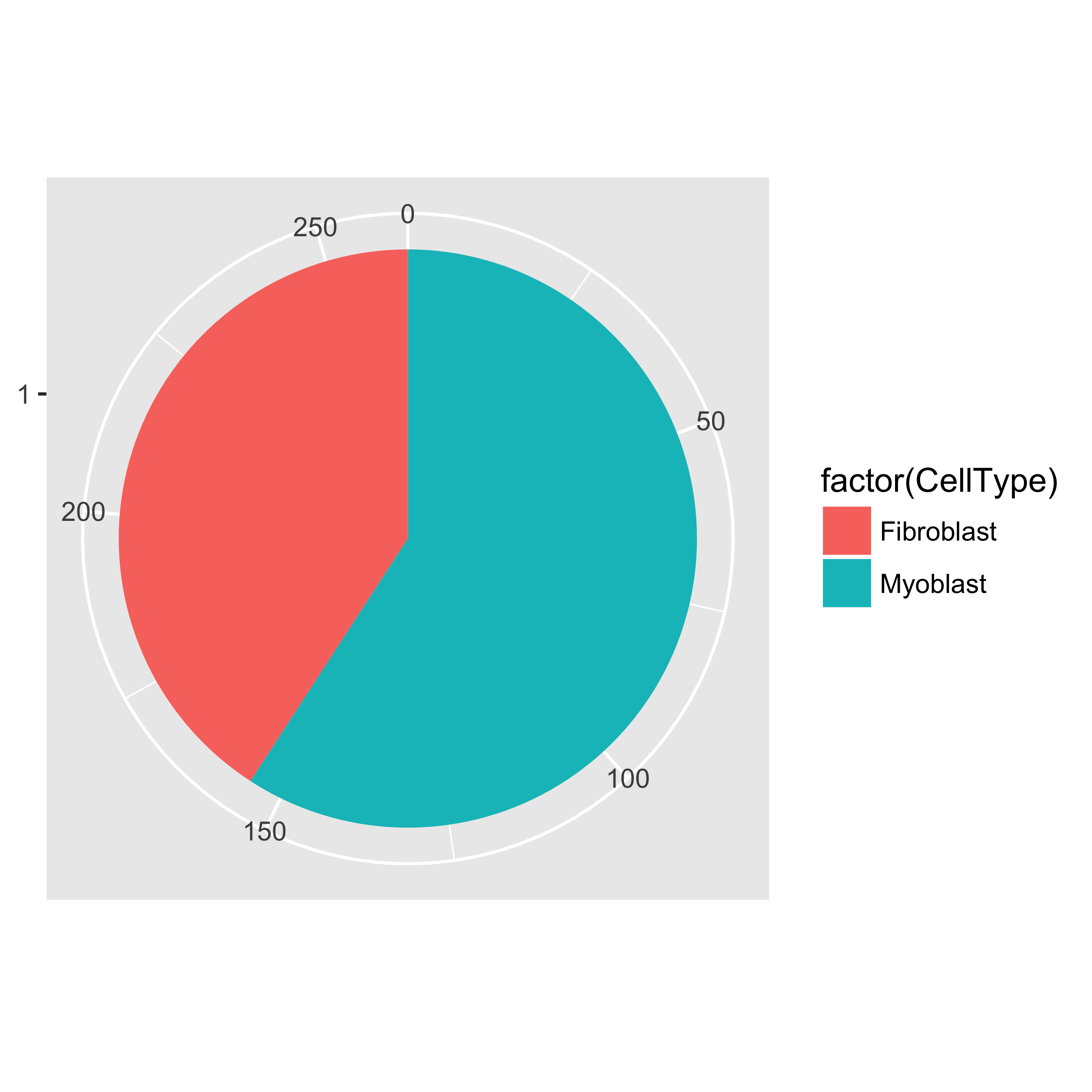
Finally, we subset the CellDataSet object to create HSMM_myo, which includes only myoblasts. We'll use this in the rest of the analysis.
switch from growth medium to differentiation mediumConstructing Single Cell Trajectories
During development, in response to stimuli, and througout life, cells transition from one functional "state" to another. Cells in different states express different sets of genes, producing a dynamic repetoire of proteins and metabolites that carry out their work. As cells move between states, undergo a process of transcriptional re-configuration, with some genes being silenced and others newly activated. These transient states are often hard to characterize because purifying cells in between more stable endpoint states can be difficult or impossible. Single-cell RNA-Seq can enable you to see these states without the need for purification. However, to do so, we must determine where each cell is the range of possible states.
Monocle introduced the strategy of using RNA-Seq for single cell trajectory analysis. Rather than purifying cells into discrete states experimentally, Monocle uses an algorithm to learn the sequence of gene expression changes each cell must go through as part of a dynamic biological process. Once it has learned the overall "trajectory" of gene expression changes, Monocle can place each cell at its proper position in the trajectory. You can then use Monocle's differential analysis toolkit to find genes regulated over the course of the trajectory, as described in the section Finding Genes that Change as a Function of Pseudotime . If there are multiple outcome for the process, Monocle will reconstruct a "branched" trajectory. These branches correspond to cellular "decisions", and Monocle provides powerful tools for identifying the genes affected by them and involved in making them. You can see how to analyze branches in the section Analyzing Branches in Single-Cell Trajectories . Monocle relies on a machine learning technique called reversed graph embedding to construct single-cell trajectories. You can read more about the theoretical foundations of Monocle's approach in the section Theory Behind Monocle , or consult the references shown at the end of the vignette.
What is pseudotime?
The ordering workflow
Before we get into the details of ordering cells along a trajectory, it's important to understand what Monocle is doing. The ordering workflow has three main steps, each of which involve a significant machine learning task.Step 1: choosing genes that define progress
Inferring a single-cell trajectory is a machine learning problem. The first step is to select the genes Monocle will use as input for its machine learning approach. This is called feature selection, and it has a major impact in the shape of the trajectory. In single-cell RNA-Seq, genes expressed at low levels are often very noisy, but some contain important information regarding the state of the cell. Monocle orders cells by examining the pattern of expression of these genes across the cell population. Monocle looks for genes that vary in "interesting" (i.e. not just noisy) ways, and uses these to structure the data. Monocle provides you with a variety of tools to select genes that will yield a robust, accurate, and biologically meaningful trajectory. You can use these tools to either perform a completely "unsupervised" analysis, in which Monocle has no forehand knowledge of which gene you consider important. Alternatively, you can make use of expert knowledge in the form of genes that are already known to define biolgical progress to shape Monocle's trajectory. We consider this mode "semi-supervised", because Monocle will augment the markers you provide with other, related genes.
Step 2: reducing the dimensionality of the data
Once we have selected the genes we will use to order the cells, Monocle applies a dimensionality reduction to the data. Monocle uses a recently developed algoithm called Reversed Graph Embedding to reduce the data's dimensionality.
Step 3: ordering the cells in pseudotime
With the expression data projected into a lower dimensional space, Monocle is ready to learn the trajectory that describes how cells transition from one state into another. Monocle assumes that the trajectory has a tree structure, with one end of it the "root", and the others the "leaves". Monocle's job is to fit the best tree it can to the data. This task is called manifold learning A cell at the beginning of the biological process starts at the root and progresses along the trunk until it reaches the first branch, if there is one. That cell must then choose a path, and moves further and further along the tree until it reaches a leaf. A cell's pseudotime value is the distance it would have to travel to get back to the root.
Trajectory step 1: choose genes that define a cell's progress
First, we must decide which genes we will use to define a cell's progress through myogenesis. We ultimately want a set of genes that increase (or decrease) in expression as a function of progress through the process we're studying.
Ideally, we'd like to use as little prior knowledge of the biology of the system under study as possible. We'd like to discover the important ordering genes from the data, rather than relying on literature and textbooks, because that might introduce bias in the ordering. We'll start with one of the simpler ways to do this, but we generally recommend a somewhat more sophisticated approach called "dpFeature".
One effective way to isolate a set of ordering genes is to simply compare the cells collected at the beginning of the process to those at the end and find the differentially expressed genes, as described above. The command below will find all genes that are differentially expressed in response to the switch from growth medium to differentiation medium:
diff_test_res <- differentialGeneTest(HSMM_myo[expressed_genes,],
              fullModelFormulaStr = "~Media")
ordering_genes <- row.names (subset(diff_test_res, qval < 0.01))
Choosing genes based on differential analysis of time points is often highly effective, but what if we don't have time series data? If the cells are asynchronously moving through our biological process (as is usually the case), Monocle can often reconstruct their trajectory from a single population captured all at the same time. Below are two methods to select genes that require no knowledge of the design of the experiment at all.
Once we have a list of gene ids to be used for ordering, we need to set them in
the HSMM object, because the next several functions will depend on
them.
Once we have a list of gene ids to be used for ordering, we need to set them in the HSMM object, because the next several functions will depend on them.
HSMM_myo <- setOrderingFilter(HSMM_myo, ordering_genes)
plot_ordering_genes(HSMM_myo)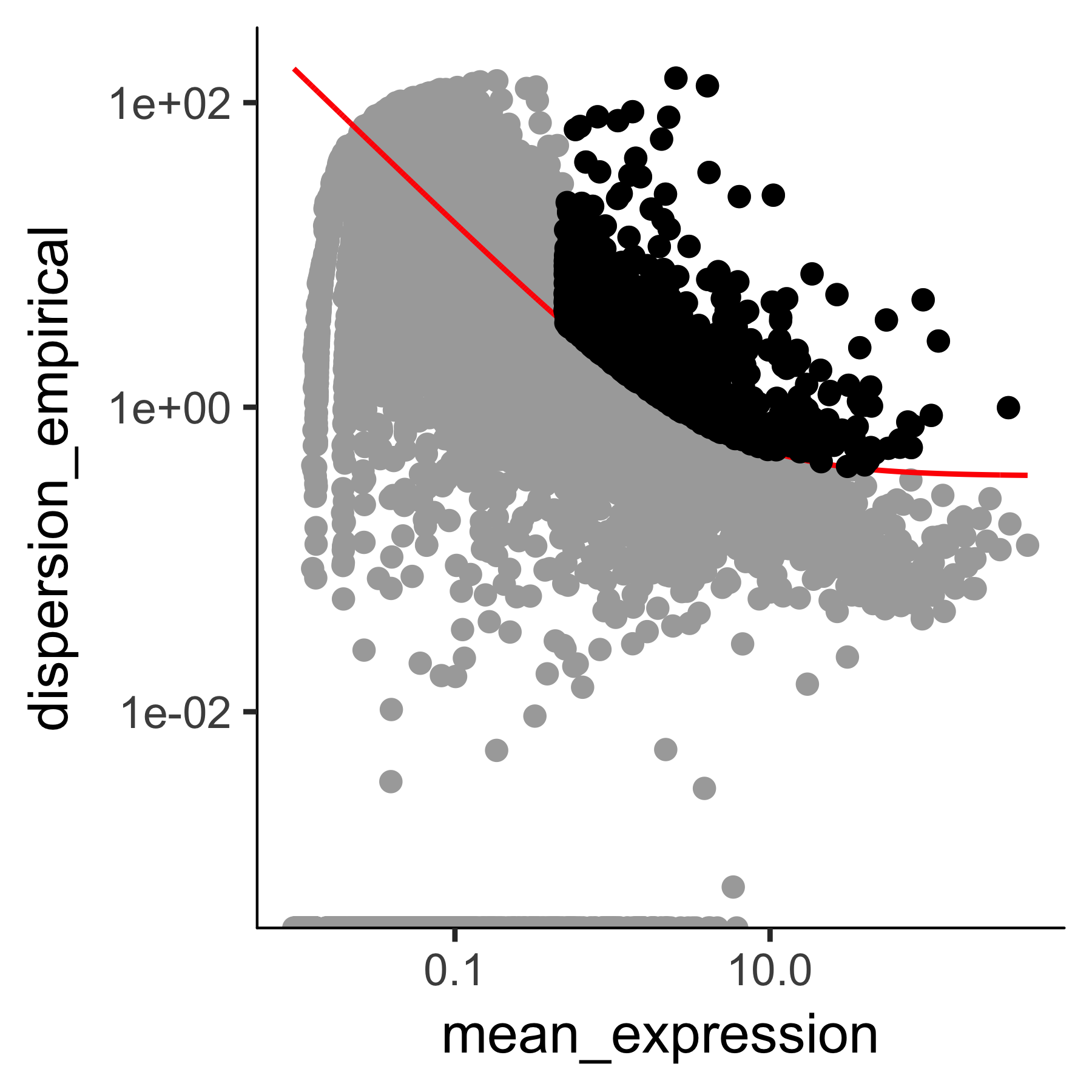
Trajectory step 2: reduce data dimensionality
Next, we will reduce the space down to one with two dimensions, which we will be
able to easily visualize and interpret while Monocle is ordering the cells.
HSMM_myo <- reduceDimension(HSMM_myo, max_components = 2,
    method = 'DDRTree')
Trajectory step 3: order cells along the trajectory
Now that the space is reduced, it's time to order the cells using the
orderCells function as shown below.
HSMM_myo <- orderCells(HSMM_myo)
Once the cells are ordered, we can visualize the trajectory in the reduced dimensional space.
plot_cell_trajectory(HSMM_myo, color_by = "Hours")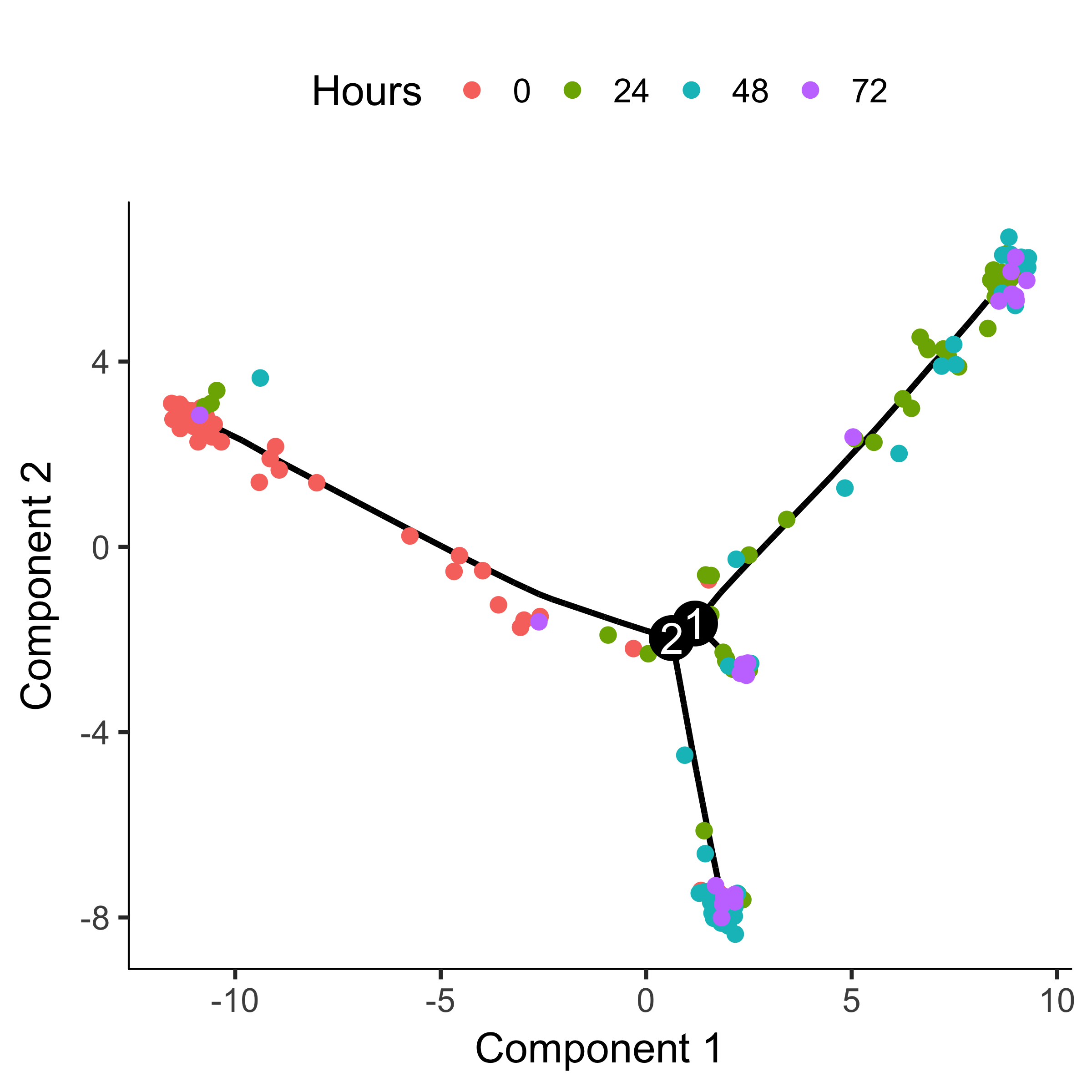
The trajectory has a tree-like structure. We can see that the cells collected at
time zero are located near one of the tips of the tree, while the others are
distributed amongst the two "branches". Monocle doesn't know a priori
which of the trajectory of the tree to call the "beginning", so we often have to
call orderCells again using the root_state argument to
specify the beginning. First, we plot the trajectory, this time coloring the
cells by "State":
plot_cell_trajectory(HSMM_myo, color_by = "State")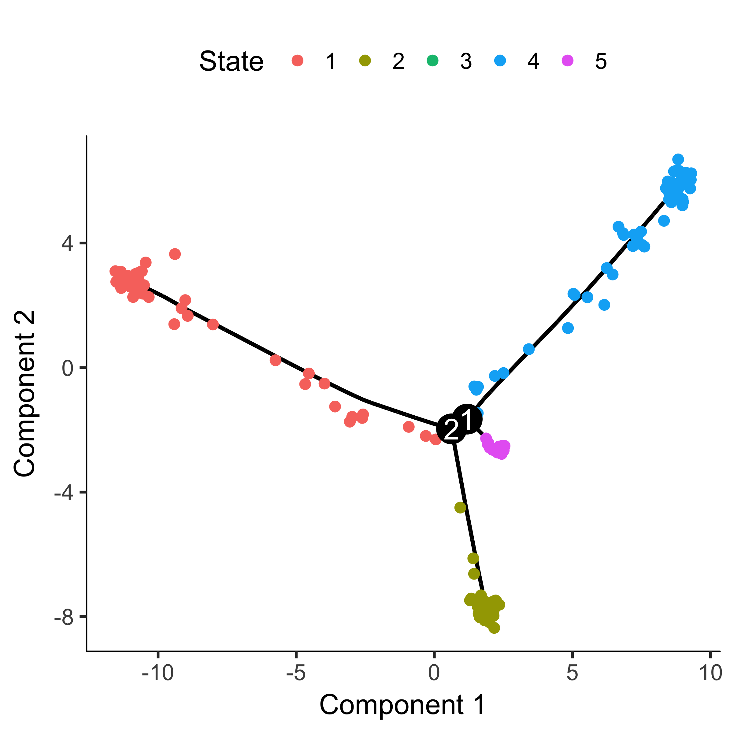
"State" is just Monocle's term for the segment of the tree. The function below
is handy for identifying the State which contains most of the cells from time
zero. We can then pass that to orderCells:
GM_state <- function(cds){
  if (length(unique(pData(cds)$State)) > 1){
    T0_counts <- table(pData(cds)$State, pData(cds)$Hours)[,"0"]
    return(as.numeric(names(T0_counts)[which
          (T0_counts == max(T0_counts))]))
  } else {
    return (1)
  }
}
HSMM_myo <- orderCells(HSMM_myo, root_state = GM_state(HSMM_myo))
plot_cell_trajectory(HSMM_myo, color_by = "Pseudotime")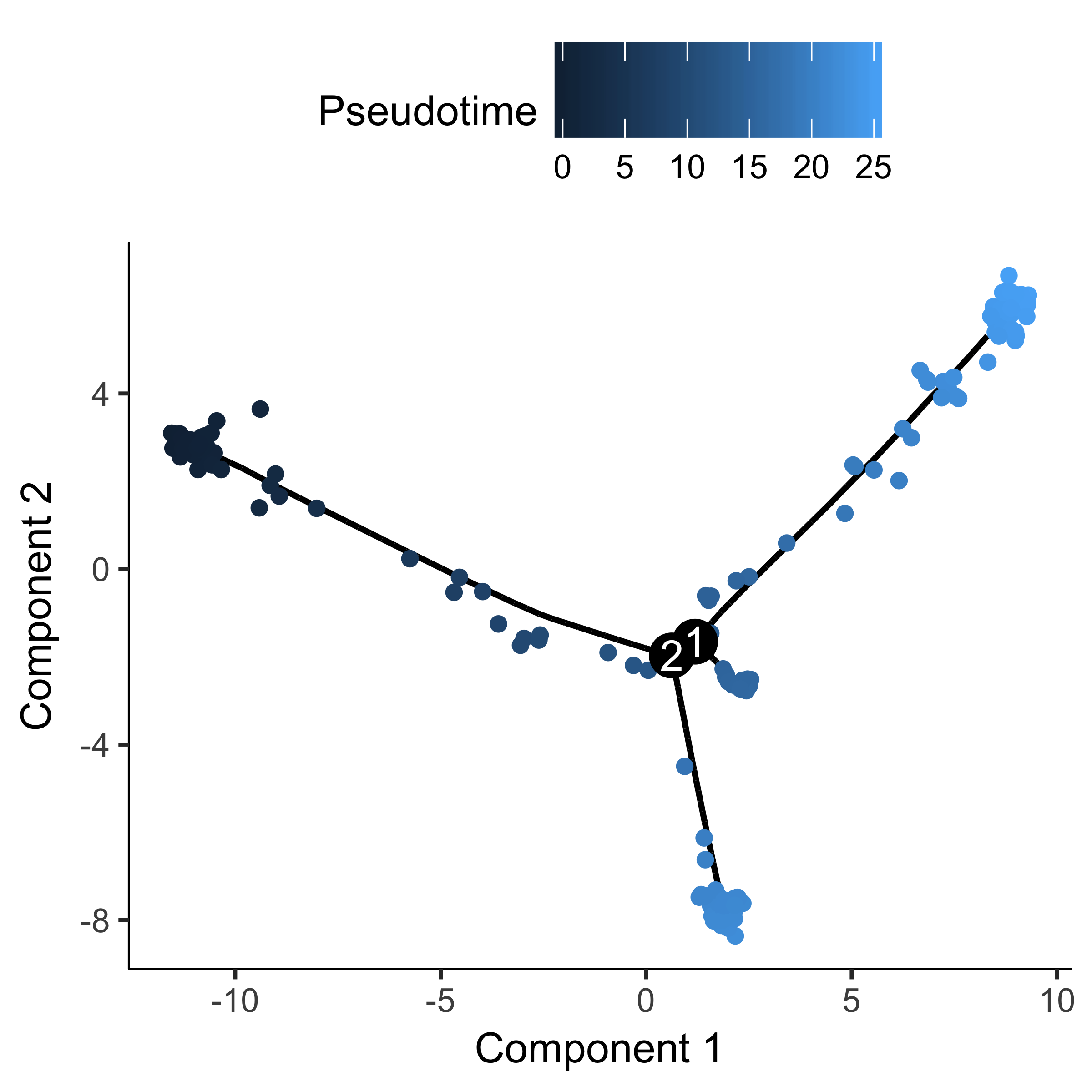
If there are a ton of states in your tree, it can be a little hard to make out where each one falls on the tree. Sometimes it can be handy to "facet" the trajectory plot so it's easier to see where each of the states are located:
plot_cell_trajectory(HSMM_myo, color_by = "State") +
    facet_wrap(~State, nrow = 1)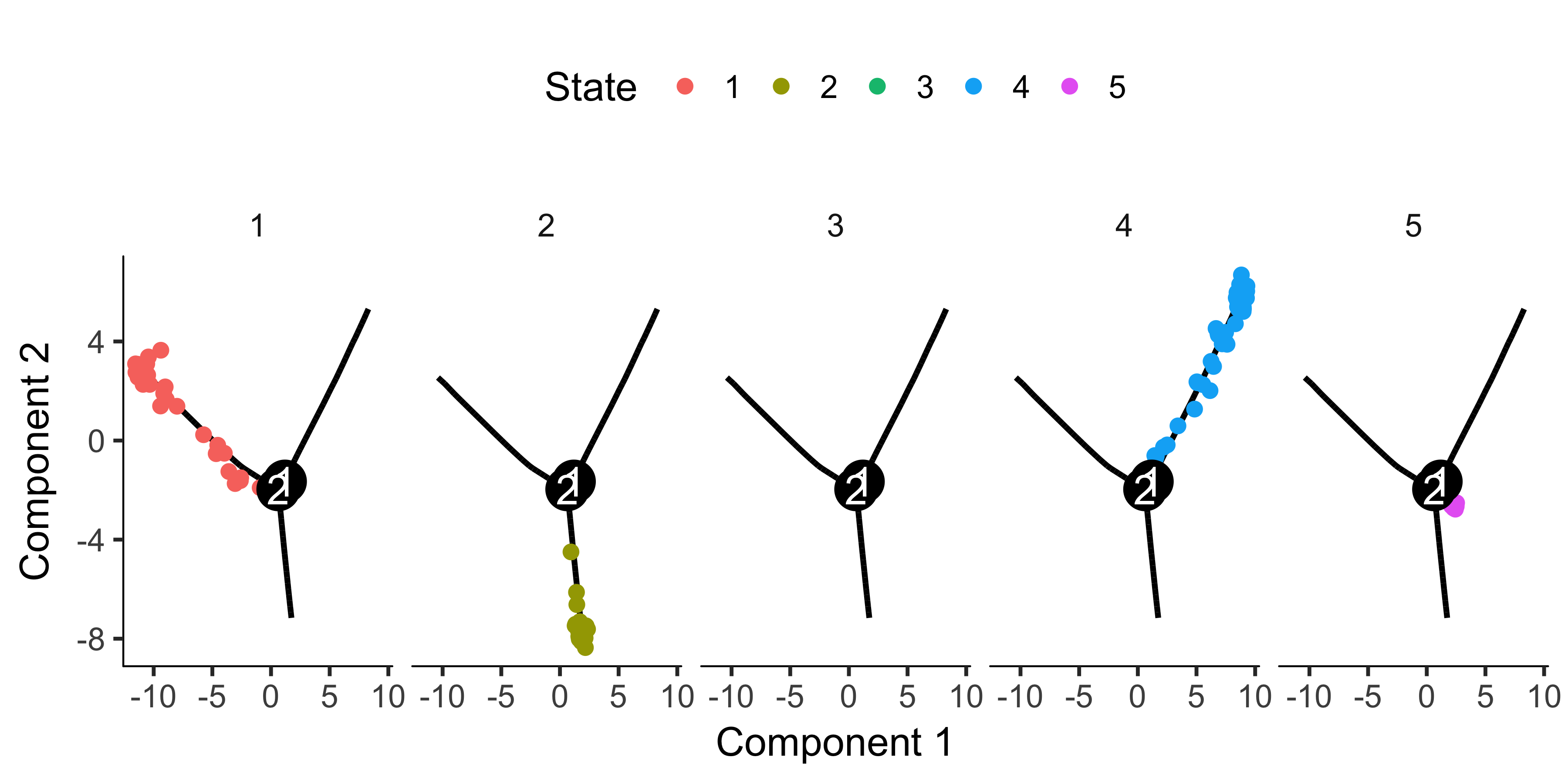
And if you don't have a timeseries, you might need to set the root based on where certain marker genes are expressed, using your biological knowledge of the system. For example, in this experiment, a highly proliferative population of progenitor cells are generating two types of post-mitotic cells. So the root should have cells that express high levels of proliferation markers. We can use the jitter plot to pick figure out which state corresponds to rapid proliferation:
blast_genes <- row.names(subset(fData(HSMM_myo),
gene_short_name %in% c("CCNB2", "MYOD1", "MYOG")))
plot_genes_jitter(HSMM_myo[blast_genes,],
    grouping = "State",
    min_expr = 0.1)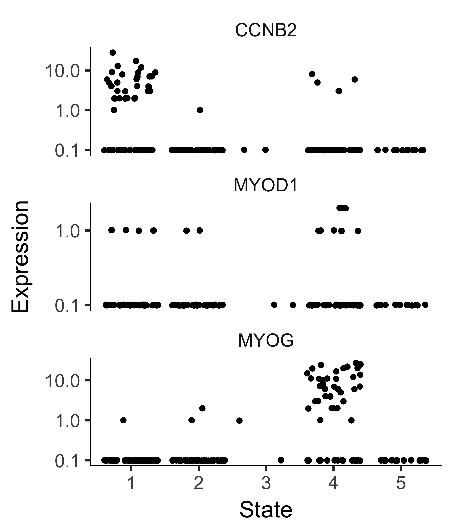
To confirm that the ordering is correct we can select a couple of markers of myogenic progress. Plotting these genes demonstrates that ordering looks good:
HSMM_expressed_genes <-  row.names(subset(fData(HSMM_myo),
num_cells_expressed >= 10))
HSMM_filtered <- HSMM_myo[HSMM_expressed_genes,]
my_genes <- row.names(subset(fData(HSMM_filtered),
          gene_short_name %in% c("CDK1", "MEF2C", "MYH3")))
cds_subset <- HSMM_filtered[my_genes,]
plot_genes_in_pseudotime(cds_subset, color_by = "Hours")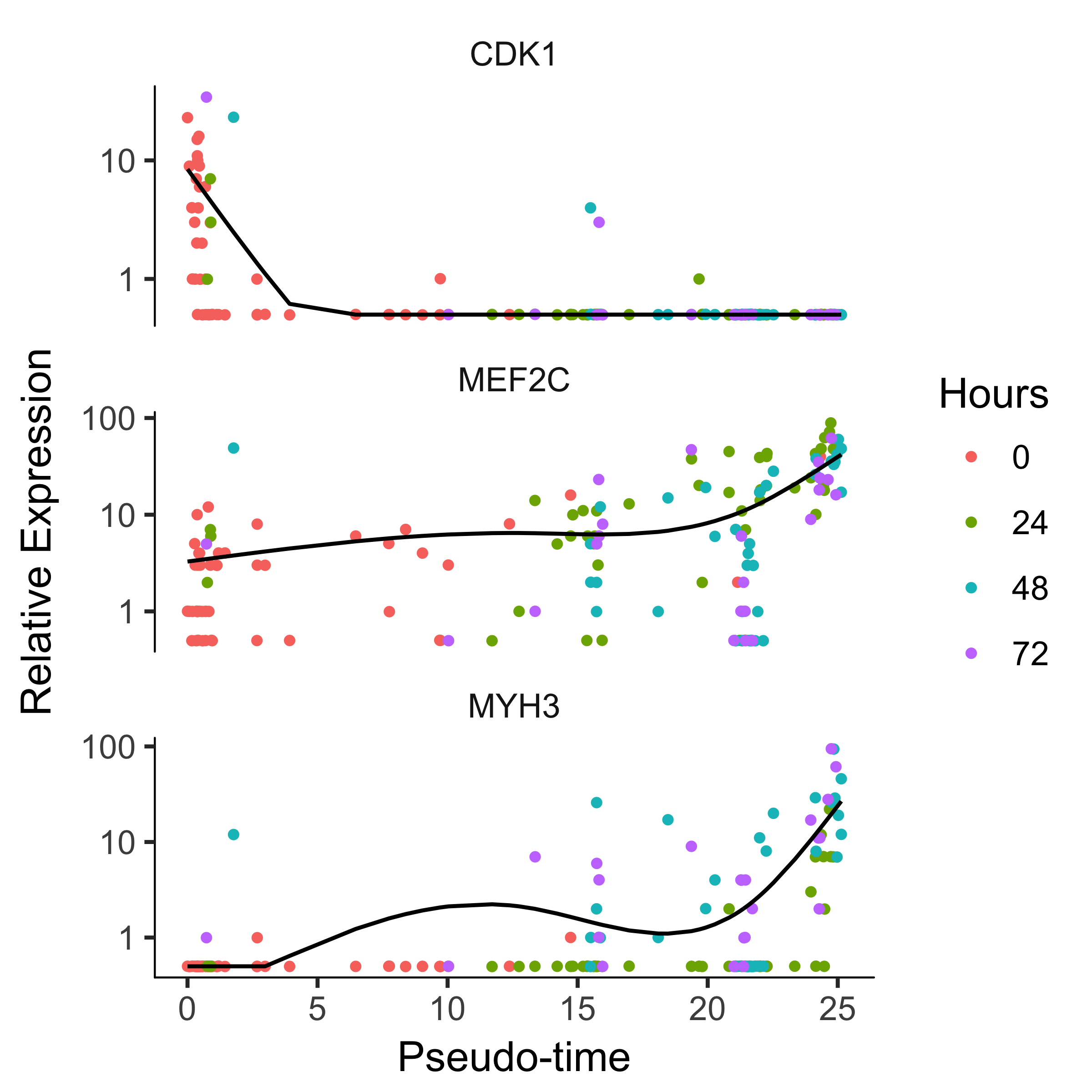
How to reverse a linear trajectory
orderCells an optional argument argument: the
reverse flag. The reverse flag tells Monocle to reverse the
orientation of the entire process as it's being discovered from the data,
so that the cells that would have been assigned to the end are instead assigned
to the beginning, and so on.
Alternative choices for ordering genes
Ordering based on genes that differ between clusters Recommended
We recommend users a order cells using genes selected by an unsupervised procedure called "dpFeature".
To use dpFeature, we first select superset of feature genes as genes expressed in at least 5% of all the cells.
HSMM_myo <- detectGenes(HSMM_myo, min_expr = 0.1)
fData(HSMM_myo)$use_for_ordering <-
    fData(HSMM_myo)$num_cells_expressed > 0.05 * ncol(HSMM_myo)
Then we will perform a PCA analysis to identify the variance explained by each PC (principal component). We can look at a scree plot and determine how many pca dimensions are wanted based on whether or not there is a significant gap between that component and the component after it. By selecting only the high loading PCs, we effectively only focus on the more interesting biological variations.
plot_pc_variance_explained(HSMM_myo, return_all = F)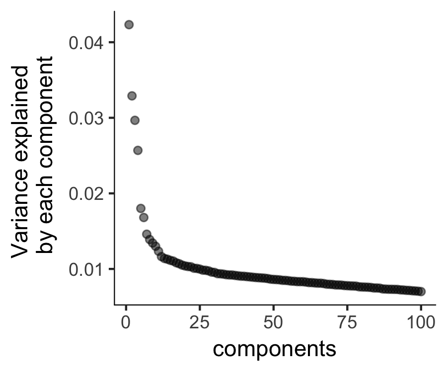
We will then run reduceDimension with t-SNE as the reduction method on those top PCs and project them further down to two dimensions.
HSMM_myo <- reduceDimension(HSMM_myo,
                              max_components = 2,
                              norm_method = 'log',
                              num_dim = 3,
                              reduction_method = 'tSNE',
                              verbose = T)
Then we can run density peak clustering to identify the clusters on the 2-D
t-SNE space. The densityPeak algorithm clusters cells based on each cell's local
density (Ρ) and the nearest distance (Δ) of a cell to another cell
with higher distance. We can set a threshold for the Ρ, Δ and define
any cell with a higher local density and distance than the thresholds as the
density peaks. Those peaks are then used to define the clusters for all cells.
By default, clusterCells choose 95% of Ρ and Δ
to define the thresholds. We can also set a number of clusters (n) we
want to cluster. In this setting, we will find the top n cells with
high Δ with Δ among the top 50% range. The default setting
often gives good clustering.
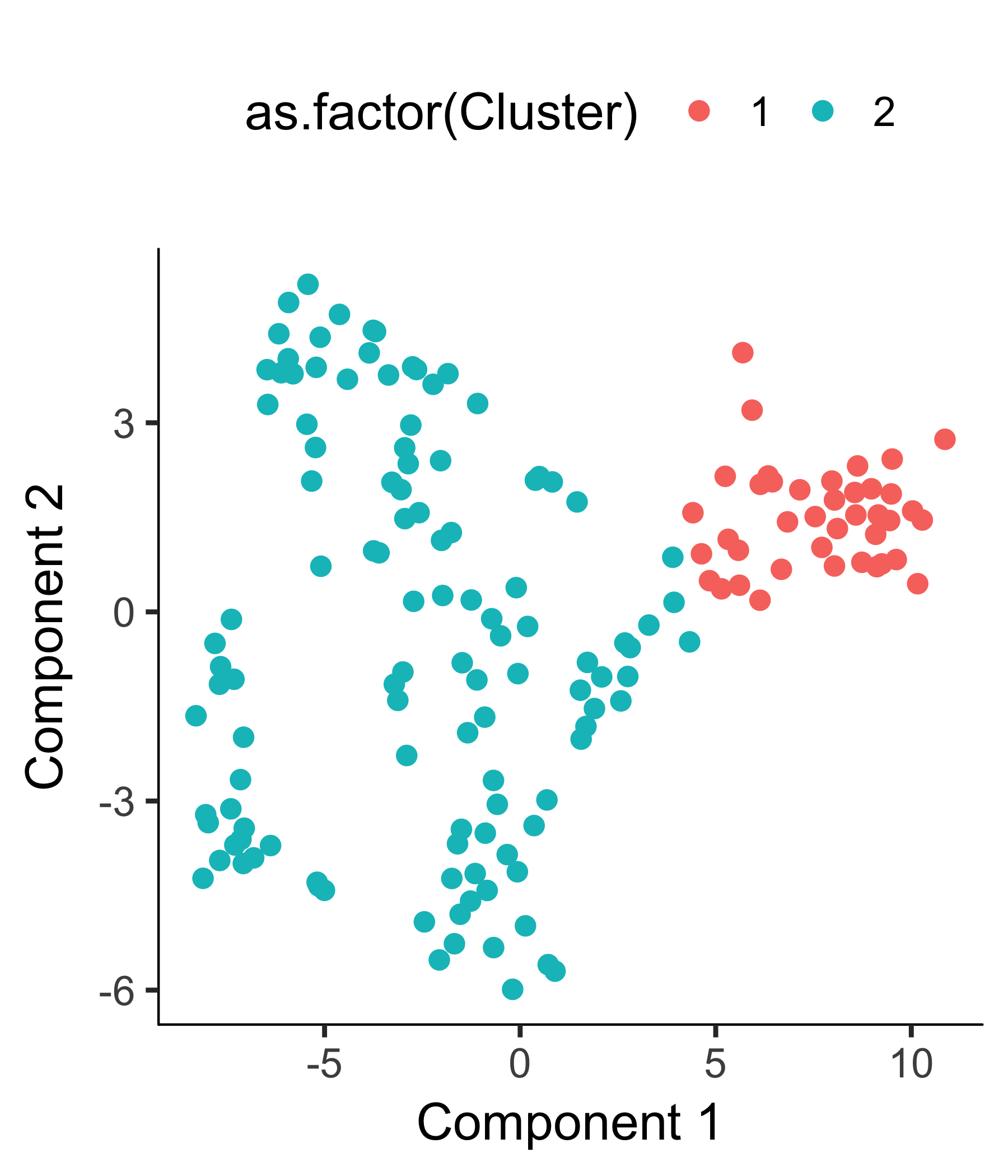
HSMM_myo <- clusterCells(HSMM_myo, verbose = F)
After the clustering, we can check the clustering results.
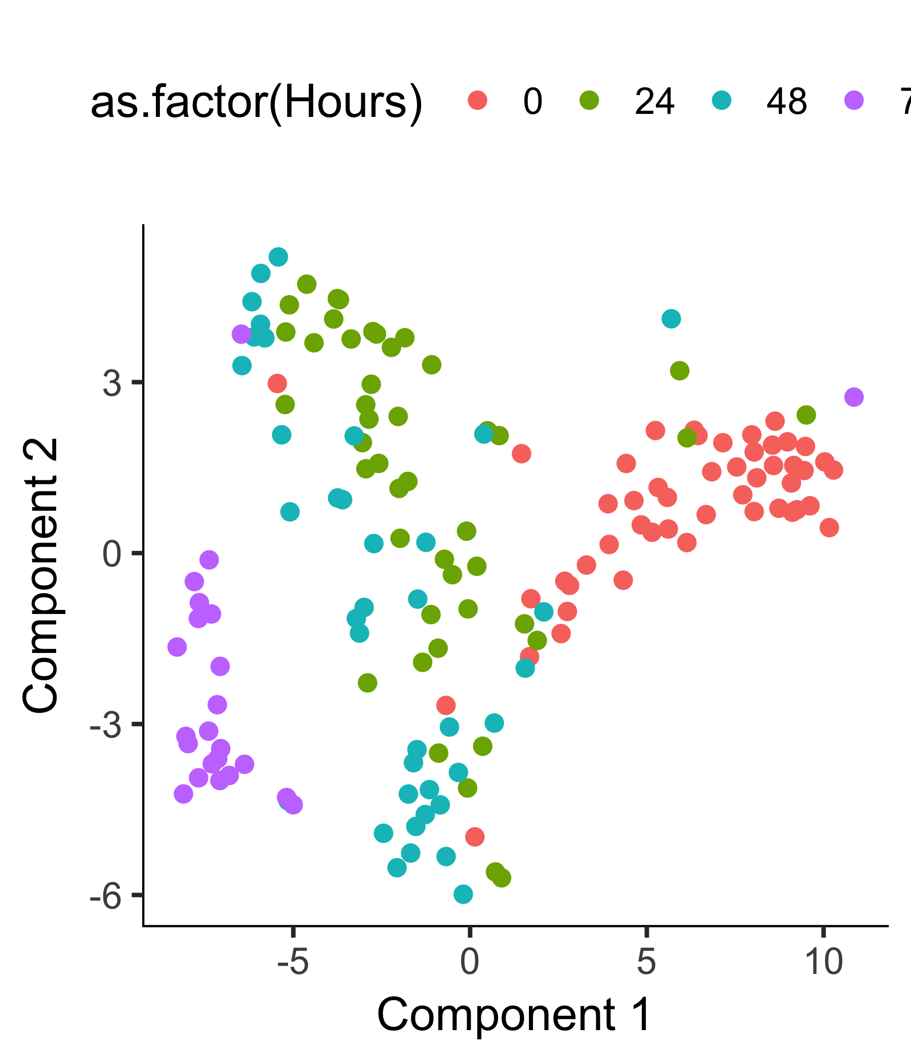
plot_cell_clusters(HSMM_myo, color_by = 'as.factor(Cluster)')
plot_cell_clusters(HSMM_myo, color_by = 'as.factor(Hours)')
We also provide the decision plot for users to check the Ρ, Δ for each cell and decide the threshold for defining the cell clusters.
plot_rho_delta(HSMM_myo, rho_threshold = 2, delta_threshold = 4 )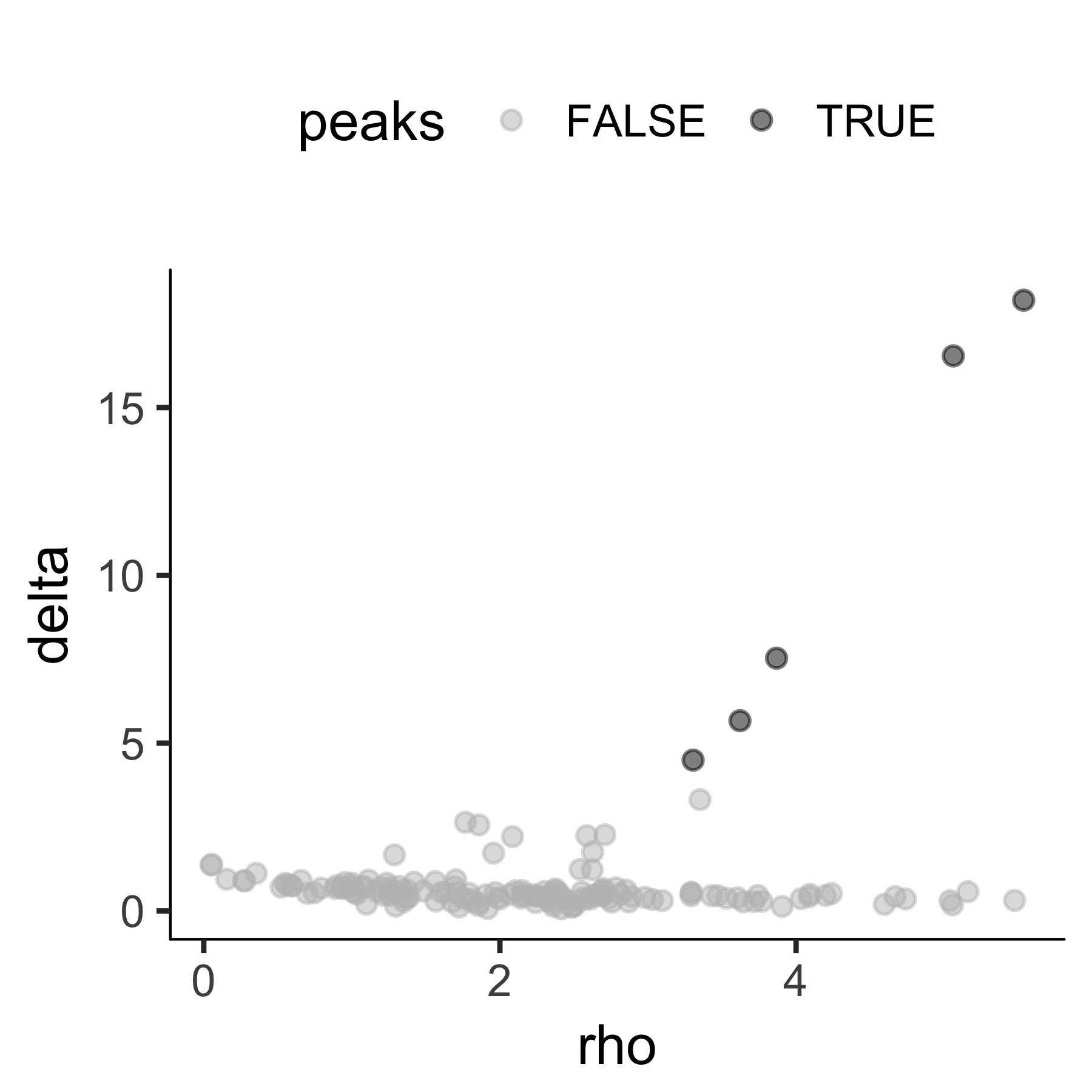
We could then re-run clustering based on the user defined threshold. To
facilitate the computation, we can set (skip_rho_sigma = T)
which enables us to skip the calculation of the Ρ, Σ.
HSMM_myo <- clusterCells(HSMM_myo,
                 rho_threshold = 2,
                 delta_threshold = 4,
                 skip_rho_sigma = T,
verbose = F)plot_cell_clusters(HSMM_myo, color_by = 'as.factor(Cluster)')
plot_cell_clusters(HSMM_myo, color_by = 'as.factor(Hours)')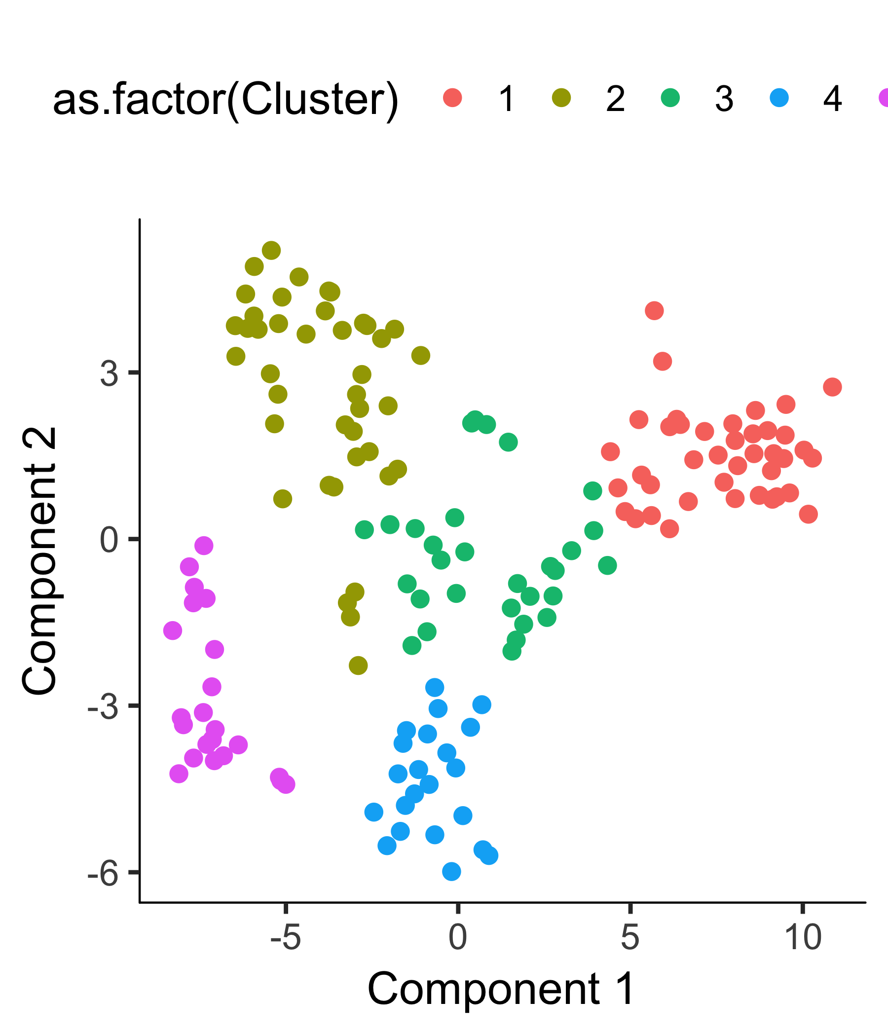

After we confirm the clustering makes sense, we can then perform differential gene expression test as a way to extract the genes that distinguish them.
clustering_DEG_genes <-
    differentialGeneTest(HSMM_myo[HSMM_expressed_genes,],
          fullModelFormulaStr = '~Cluster',
          cores = 1)
We will then select the top 1000 significant genes as the ordering genes.
HSMM_ordering_genes <-
    row.names(clustering_DEG_genes)[order(clustering_DEG_genes$qval)][1:1000]

HSMM_myo <-
    setOrderingFilter(HSMM_myo,
        ordering_genes = HSMM_ordering_genes)

HSMM_myo <-
    reduceDimension(HSMM_myo, method = 'DDRTree')

HSMM_myo <-
    orderCells(HSMM_myo)

HSMM_myo <-
    orderCells(HSMM_myo, root_state = GM_state(HSMM_myo))

plot_cell_trajectory(HSMM_myo, color_by = "Hours")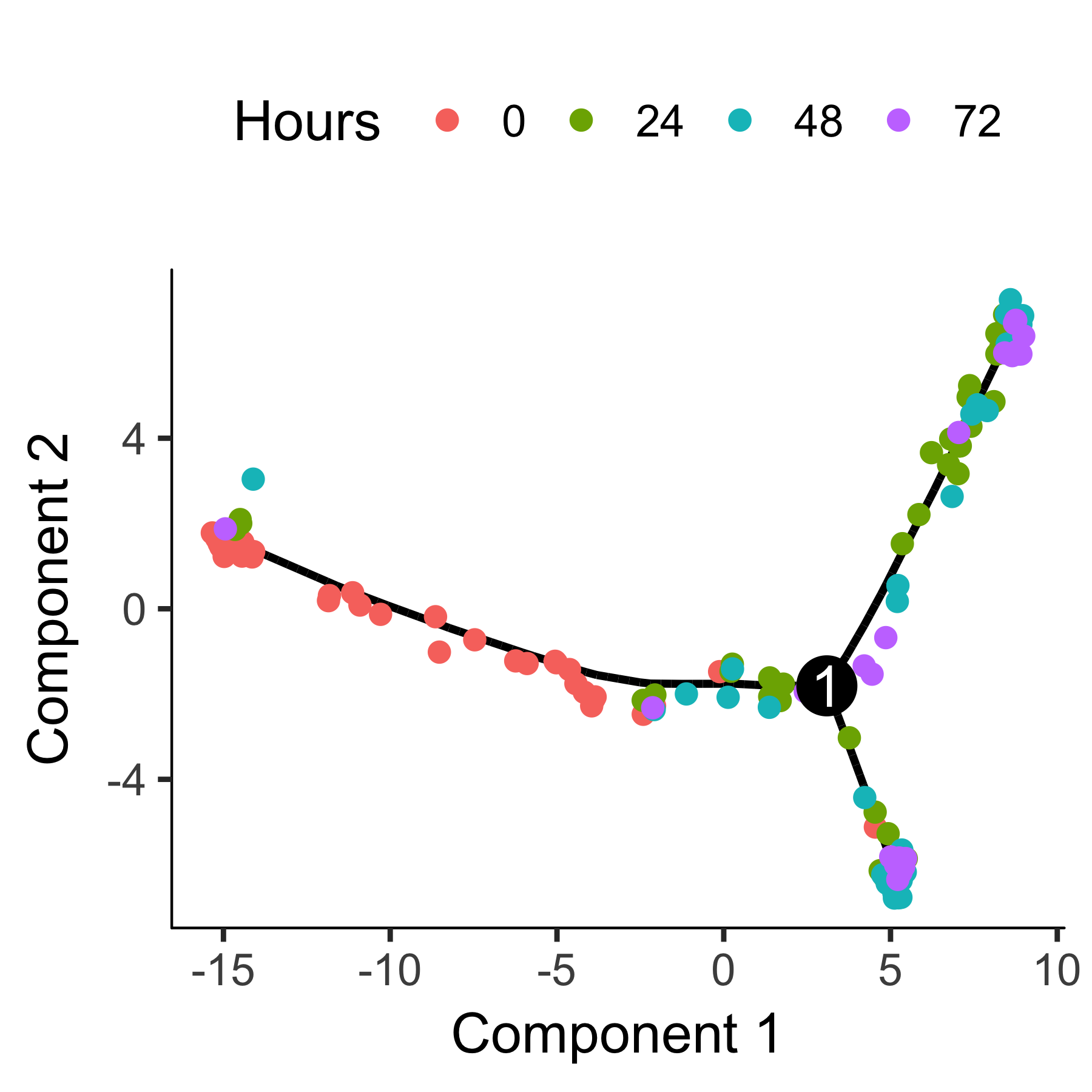
Selecting genes with high dispersion across cells Alternative
Genes that vary a lot are often highly informative for identifying cell subpopulations or ordering cells along a trajectory. In RNA-Seq, a gene's variance typically depends on its mean, so we have to be a bit careful about how we select genes based on their variance.
disp_table <- dispersionTable(HSMM_myo)
ordering_genes <- subset(disp_table,
                  mean_expression >= 0.5 &
                  dispersion_empirical >= 1 * dispersion_fit)$gene_id
Ordering cells using known marker genes Alternative
Unsupervised ordering is desirable because it avoids introducing bias into the analysis. However, unsupervised machine learning will sometimes fix on a strong feature of the data that's not the focus of your experiment. For example, where each cell is in the cell cycle has a major impact on the shape of the trajectory when you use unsupervised learning. But what if you wish to focus on cycle-independent effects in your biological process? Monocle's "semi-supervised" ordering mode can help you focus on the aspects of the process you're interested in.
Ordering your cells in a semi-supervised manner is very simple. You first define genes that mark progress using the CellTypeHierchy system, very similar to how we used it for cell type classification. Then, you use it to select ordering genes that co-vary with these markers. Finally, you order the cell based on these genes just as we do in unsupervised ordering. So the only difference between unsupervised and semi-supervised ordering is in which genes we use for ordering.
As we saw before, myoblasts begin differnentation by exiting the cell cycle and
then proceed through a sequence of regulatory events that leads to expression of
some key muscle-specific proteins needed for contraction. We can mark cycling
cells with cyclin B2 (CCNB2) and recognize myotubes as those cells
expressed high levels of myosin heavy chain 3 (MYH3).
CCNB2_id <-
    row.names(subset(fData(HSMM_myo), gene_short_name == "CCNB2"))
MYH3_id <-
    row.names(subset(fData(HSMM_myo), gene_short_name == "MYH3"))

cth <- newCellTypeHierarchy()

cth <- addCellType(cth,
                   "Cycling myoblast",
                   classify_func = function(x) { x[CCNB2_id,] >= 1 })

cth <- addCellType(cth,
                   "Myotube",
                   classify_func = function(x) { x[MYH3_id,] >= 1 })

cth <- addCellType(cth,
                   "Reserve cell",
                   classify_func =
                function(x) { x[MYH3_id,] == 0 & x[CCNB2_id,] == 0 })

HSMM_myo <- classifyCells(HSMM_myo, cth)marker_diff <- markerDiffTable(HSMM_myo[HSMM_expressed_genes,],
cth,
cores = 1)
#semisup_clustering_genes <-
#row.names(subset(marker_diff, qval < 0.05))
semisup_clustering_genes <-
row.names(marker_diff)[order(marker_diff$qval)][1:1000]
Using the top 1000 genes for ordering produces a trajectory that's highly similar to the one we obtained with unsupervised methods, but it's a little "cleaner".
HSMM_myo <- setOrderingFilter(HSMM_myo, semisup_clustering_genes)
#plot_ordering_genes(HSMM_myo)
HSMM_myo <- reduceDimension(HSMM_myo, max_components = 2,
    method = 'DDRTree', norm_method = 'log')
HSMM_myo <- orderCells(HSMM_myo)
HSMM_myo <- orderCells(HSMM_myo, root_state = GM_state(HSMM_myo))
plot_cell_trajectory(HSMM_myo, color_by = "CellType") +
    theme(legend.position = "right")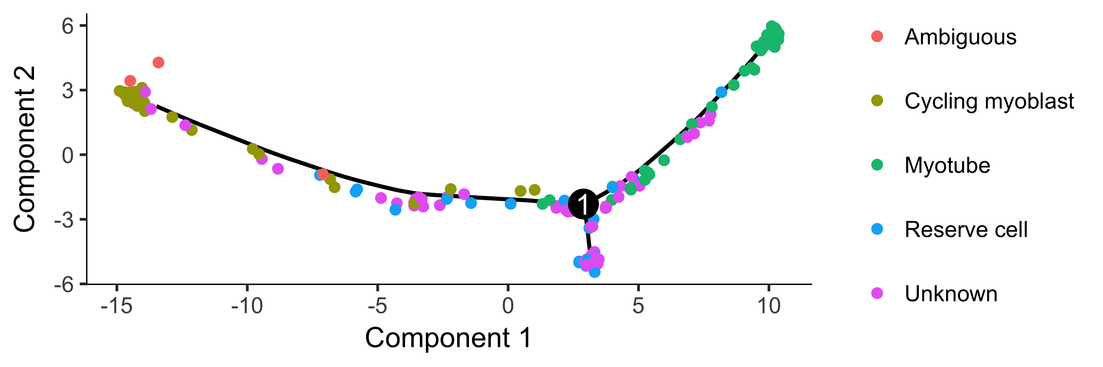
To confirm that the ordering is correct, we can select a couple of markers of myogenic progress. In this experiment, one of the branches corresponds to cells that successfully fuse to form myotubes, and the other to those that fail to fully differentiate. We will exclude the latter for now, but you can learn more about tools for dealing with branched trajectories in the section Analyzing Branches in Single-Cell Trajectories .
HSMM_filtered <- HSMM_myo[HSMM_expressed_genes,]

my_genes <- row.names(subset(fData(HSMM_filtered),
                gene_short_name %in% c("CDK1", "MEF2C", "MYH3")))

cds_subset <- HSMM_filtered[my_genes,]
plot_genes_branched_pseudotime(cds_subset,
                       branch_point = 1,
                       color_by = "Hours",
                       ncol = 1)
Differential Expression Analysis
Differential gene expression analysis is a common task in RNA-Seq experiments. Monocle can help you find genes that are differentially expressed between groups of cells and assesses the statistical signficance of those changes. These comparisons require that you have a way to collect your cells into two or more groups. These groups are defined by columns in the phenoData table of each CellDataSet. Monocle will assess the signficance of each gene's expression level across the different groups of cells.Basic Differential Analysis
Performing differential expression analysis on all genes in the human genome can take a substantial amount of time. For a dataset as large as the myoblast data from [1], which contains several hundred cells, the analysis can take several hours on a single CPU. Let's select a small set of genes that we know are important in myogenesis to demonstrate Monocle's capabilities:marker_genes <- row.names(subset(fData(HSMM_myo),
gene_short_name %in% c("MEF2C", "MEF2D", "MYF5",
"ANPEP", "PDGFRA","MYOG",
"TPM1", "TPM2", "MYH2",
"MYH3", "NCAM1", "TNNT1",
"TNNT2", "TNNC1", "CDK1",
"CDK2", "CCNB1", "CCNB2",
"CCND1", "CCNA1", "ID1")))In the myoblast data, the cells collected at the outset of the experiment were cultured in "growth medium" (GM) to prevent them from differentiating. After they were harvested, the rest of the cells were switched over to "differentiation medium" (DM) to promote differentiation. Let us have monocle find which of the genes above are affected by this switch:
diff_test_res <- differentialGeneTest(HSMM_myo[marker_genes,],
                                      fullModelFormulaStr = "~Media")

# Select genes that are significant at an FDR < 10%
sig_genes <- subset(diff_test_res, qval < 0.1)

sig_genes[,c("gene_short_name", "pval", "qval")]
So most of the 22 genes are significant at a 10% false discovery rate! This is not surprising, as most of the above genes are highly relevant in myogenesis. Monocle also provides some easy ways to plot the expression of a small set of genes grouped by the factors you use during differential analysis. This helps you visualize the differences revealed by the tests above. One type of plot is a "jitter" plot.
MYOG_ID1 <- HSMM_myo[row.names(subset(fData(HSMM_myo),
              gene_short_name %in% c("MYOG", "CCNB2"))),]
plot_genes_jitter(MYOG_ID1, grouping = "Media", ncol= 2)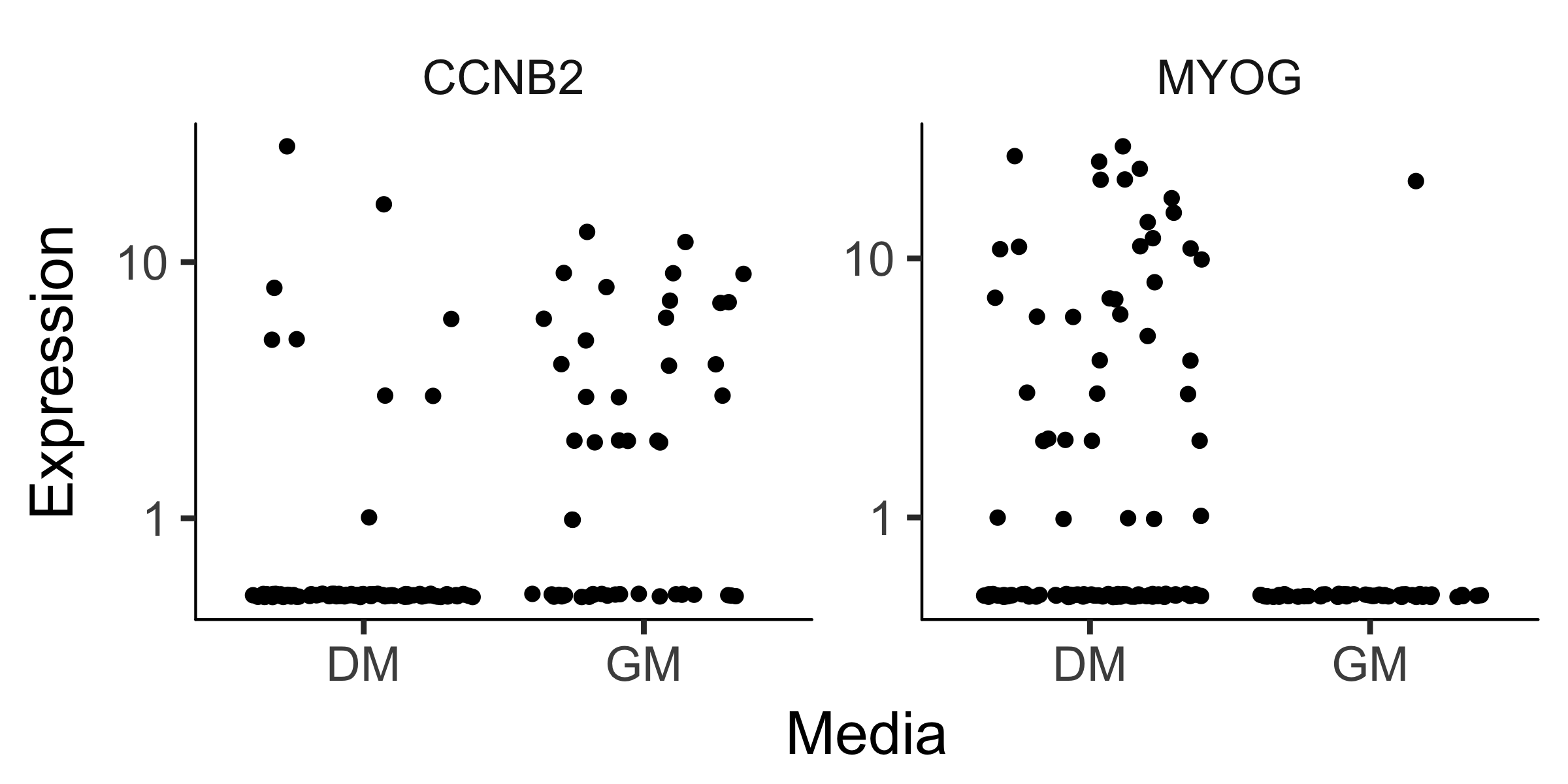
Note that we can control how to layout the genes in the plot by specifying
the number of rows and columns. See the man page on
plot_genes_jitter for more details on controlling its layout. Most
if not all of Monocle's plotting routines return a plot object from the
ggplot2 package. This package uses a grammar of graphics to control
various aspects of a plot, and makes it easy to customize how your data is
presented. See the ggplot2 book [5] for more details.
In this section, we'll explore how to use Monocle to find genes that are differentially expressed according to several different criteria. First, we'll look at how to use our previous classification of the cells by type to find genes that distinguish fibroblasts and myoblasts. Second, we'll look at how to find genes that are differentially expressed as a function of pseudotime, such as those that become activated or repressed during differentiation. Finally, you'll see how to perform multi-factorial differential analysis, which can help subtract the effects of confounding variables in your experiment.
To keep the vignette simple and fast, we'll be working with small sets of genes. Rest assured, however, that Monocle can analyze many thousands of genes even in large experiments, making it useful for discovering dynamically regulated genes during the biological process you're studying.
Finding Genes that Distinguish Cell Type or State
During a dynamic biological process such as differentiation, cells might assume distinct intermediate or final states. Recall that earlier we distinguished myoblasts from contaminating fibroblasts on the basis of several key markers. Let's look at several other genes that should distinguish between fibroblasts and myoblasts.
to_be_tested <- row.names(subset(fData(HSMM),
              gene_short_name %in% c("UBC", "NCAM1", "ANPEP")))
cds_subset <- HSMM[to_be_tested,]
To test the effects of CellType on gene expression, we simply
call differentialGeneTest on the genes we've selected.
However, we have to specify a model formula in the call to tell Monocle that we care about genes with expression levels that depends on CellType. Monocle's differential expression analysis works essentially by fitting two models to the expression values for each gene, working through each gene independently. The first of the two models is called the full model. This model is essentially a way of predicting the expression value of each gene in a given cell knowing only whether that cell is a fibroblast or a myoblast. The second model, called the reduced model, does the same thing, but it doesn't know the CellType for each cell. It has to come up with a reasonable prediction of the expression value for the gene that will be used for all the cells. Because the full model has more information about each cell, it will do a better job of predicting the expression of the gene in each cell. The question Monocle must answer for each gene is how much better the full model's prediction is than the reduced model's. The greater the improvement that comes from knowing the CellType of each cell, the more significant the differential expression result. This is a common strategy in differential analysis, and we leave a detailed statistical exposition of such methods to others.
To set up the test based on CellType, we simply call differentialGeneTest with a string specifying fullModelFormulaStr. We don't have to specify the reduced model in this case, because the default of ~1 is what we want here.
diff_test_res <- differentialGeneTest(cds_subset,
                    fullModelFormulaStr = "~CellType")
diff_test_res[,c("gene_short_name", "pval", "qval")]
Note that all the genes are significantly differentially expressed as a function of CellType except the housekeeping gene TBP, which we're using a negative control. However, we don't know which genes correspond to myoblast-specific genes (those more highly expressed in myoblasts versus fibroblast specific genes. We can again plot them with a jitter plot to see:
plot_genes_jitter(cds_subset,
                  grouping = "CellType",
                  color_by = "CellType",
                  nrow= 1,
                  ncol = NULL,
                  plot_trend = TRUE)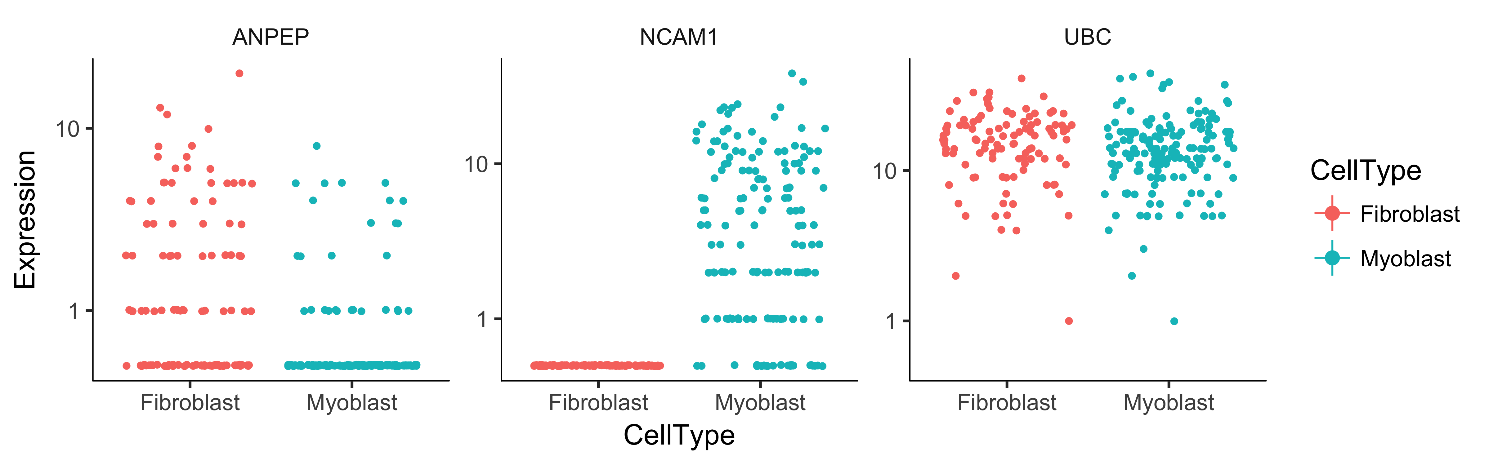
We could also simply compute summary statistics such as mean or median expression level on a per-CellType basis to see this, which might be handy if we are looking at more than a handful of genes. Of course, we could test for genes that change as a function of Hours to find time-varying genes, or Media to identify genes that are responsive to the serum switch. In general, model formulae can contain terms in the pData table of the CellDataSet.
ThedifferentialGeneTest function is actually quite simple "under the hood". The call above is equivalent to:
full_model_fits <-
    fitModel(cds_subset,  modelFormulaStr = "~CellType")
reduced_model_fits <- fitModel(cds_subset, modelFormulaStr = "~1")
diff_test_res <- compareModels(full_model_fits, reduced_model_fits)
diff_test_res
Occassionally, as we'll see later, it's useful to be able to call fitModel directly.
pData table, including those columns that are added by Monocle in other analysis steps. For example, if you use clusterCells, you can test for genes that differ between clusters by using Cluster as your model formula.
Finding Genes that Change as a Function of Pseudotime
Monocle's main job is to put cells in order of progress through a biological process (such as cell differentiation) without knowing which genes to look at ahead of time. Once it's done so, you can analyze the cells to find genes that changes as the cells make progress. For example, you can find genes that are significantly upregulated as the cells "mature". Let's look at a panel of genes important for myogenesis:
Monocle's main job is to put cells in order of progress through a biological process (such as cell differentiation) without knowing which genes to look at ahead of time. Once it's done so, you can analyze the cells to find genes that changes as the cells make progress. For example, you can find genes that are significantly upregulated as the cells "mature". Let's look at a panel of genes important for myogenesis:
to_be_tested <- row.names(subset(fData(HSMM),
gene_short_name %in% c("MYH3", "MEF2C", "CCNB2", "TNNT1")))
cds_subset <- HSMM_myo[to_be_tested,]
Again, we'll need to specify the model we want to use for differential analysis. This model will be a bit more complicated than the one we used to look at the differences between CellType. Monocle assigns each cell a "pseudotime" value, which records its progress through the process in the experiment. The model can test against changes as a function of this value. Monocle uses the VGAM package to model a gene's expression level as a smooth, nonlinear function of pseudotime.
diff_test_res <- differentialGeneTest(cds_subset,
fullModelFormulaStr = "~sm.ns(Pseudotime)")sm.ns function states that Monocle should fit a natural spline through the expression values to help it describe the changes in expression as a function of progress.
We'll see what this trend looks like in just a moment. Other smoothing functions are available.
Once again, let's add in the gene annotations so it's easy to see which genes are significant.
diff_test_res[,c("gene_short_name", "pval", "qval")]
plot_genes_in_pseudotime.
This function has a number of cosmetic options you can use to control the layout and appearance of your plot.
plot_genes_in_pseudotime(cds_subset, color_by = "Hours")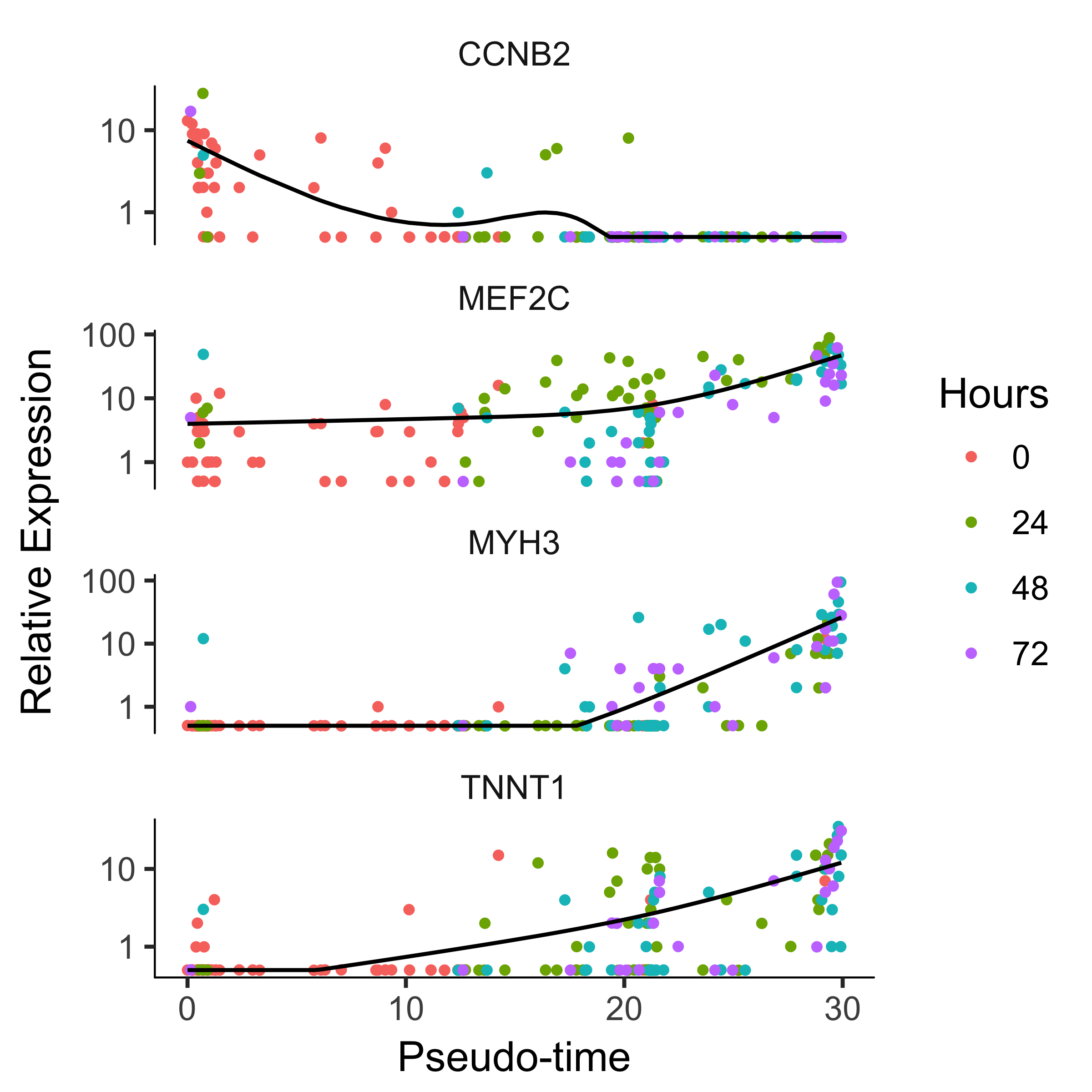
Clustering Genes by Pseudotemporal Expression Pattern
A common question that arises when studying time-series gene expression studies is: "which genes follow similar kinetic trends"?
Monocle can help you answer this question by grouping genes that have similar trends, so you can analyze these groups to see what they have in common.
Monocle provides a convenient way to visualize all pseudotime-dependent genes. The function
plot_pseudotime_heatmap takes a CellDataSet object (usually containing a only subset of significant genes)
and generates smooth expression curves much like plot_genes_in_pseudotime. Then, it clusters these genes
and plots them using the pheatmap package. This allows you to visualize modules of genes that
co-vary across pseudotime.
diff_test_res <- differentialGeneTest(HSMM_myo[marker_genes,],
              fullModelFormulaStr = "~sm.ns(Pseudotime)")
sig_gene_names <- row.names(subset(diff_test_res, qval < 0.1))
plot_pseudotime_heatmap(HSMM_myo[sig_gene_names,],
                num_clusters = 3,
                cores = 1,
                show_rownames = T)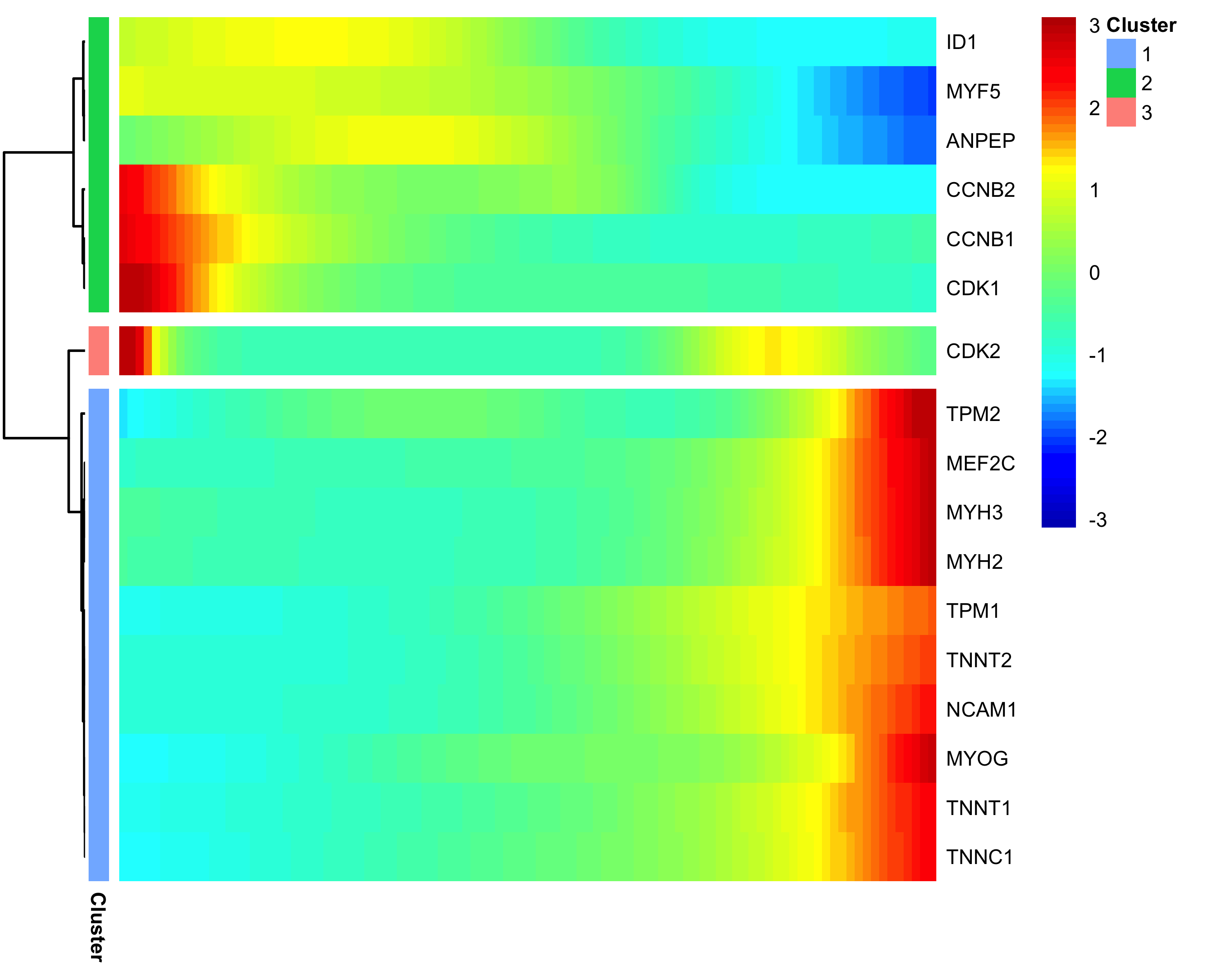
Multi-Factorial Differential Expression Analysis
Monocle can perform differential analysis in the presence of multiple factors, which can help you subtract some factors to see the effects of others. In the simple example below, Monocle tests three genes for differential expression between myoblasts and fibroblasts, while subtracting the effect of Hours, which encodes the day on which each cell was collected. To do this, we must specify both the full model and the reduced model. The full model captures the effects of both CellType and Hours, while the reduced model only knows about Hours.
When we plot the expression levels of these genes, we can modify the resulting object returned by plot_genes_jitter to allow them to have independent y-axis ranges, to better highlight the differences between cell states.
to_be_tested <-
    row.names(subset(fData(HSMM),
        gene_short_name %in% c("TPM1", "MYH3", "CCNB2", "GAPDH")))

cds_subset <- HSMM[to_be_tested,]

diff_test_res <- differentialGeneTest(cds_subset,
                        fullModelFormulaStr = "~CellType + Hours",
                        reducedModelFormulaStr = "~Hours")
diff_test_res[,c("gene_short_name", "pval", "qval")]
plot_genes_jitter(cds_subset,
    grouping = "Hours", color_by = "CellType", plot_trend = TRUE) +
        facet_wrap( ~ feature_label, scales= "free_y")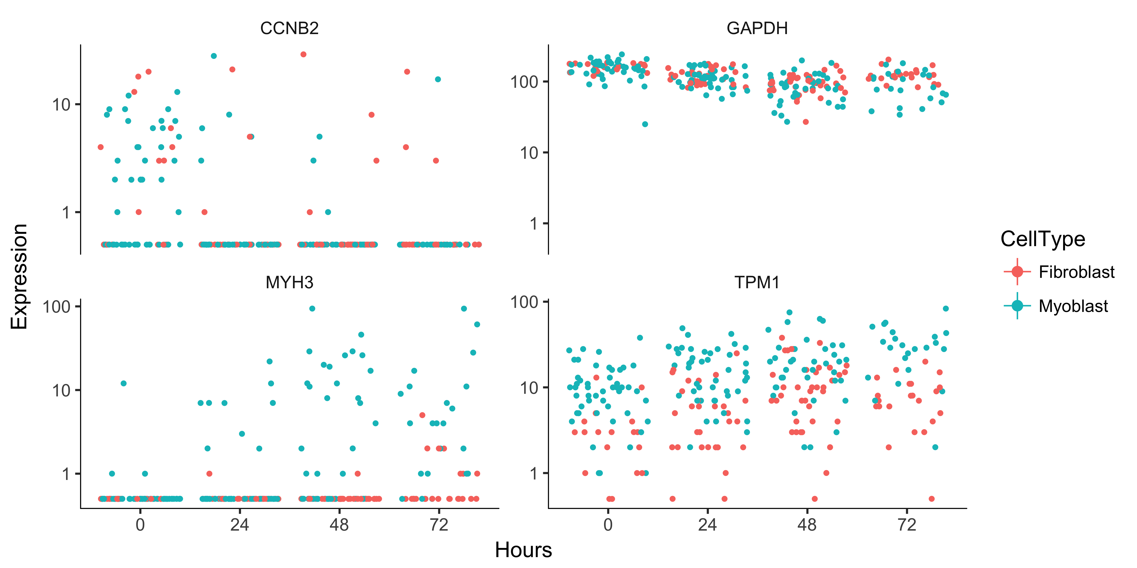
Analyzing Branches in Single-Cell Trajectories
Often, single-cell trajectories include branches. The branches occur because cells execute alternative gene expression programs. Branches appear in trajectories during development, when cells make fate choices: one developmental lineage proceeds down one path, while the other lineage produces a second path. Monocle contains extensive functionality for analyzing these branching events.
Consider the experiment performed by Steve Quake's lab by Barbara Treutlein and colleages, who captured cells from the developing mouse lung. They captured cells early in development, later when the lung contains both major types of epithelial cells (AT1 and AT2), and cells right about to make the decision to become either AT1 or AT2. Monocle can reconstruct this process as a branched trajectory, allow you to analyze the decision point in great detail. The figure below shows the trajectory Monocle reconstructs using some of their data. There is a single branch, labeled "1". What genes change as cells pass from the early developmental stage the top left of the tree through the branch? What genes are differentially expressed between the branches? To answer this question, Monocle provides you with a special statistical test: branched expression analysis modeling, or BEAM.lung <- load_lung()
plot_cell_trajectory(lung, color_by = "Time")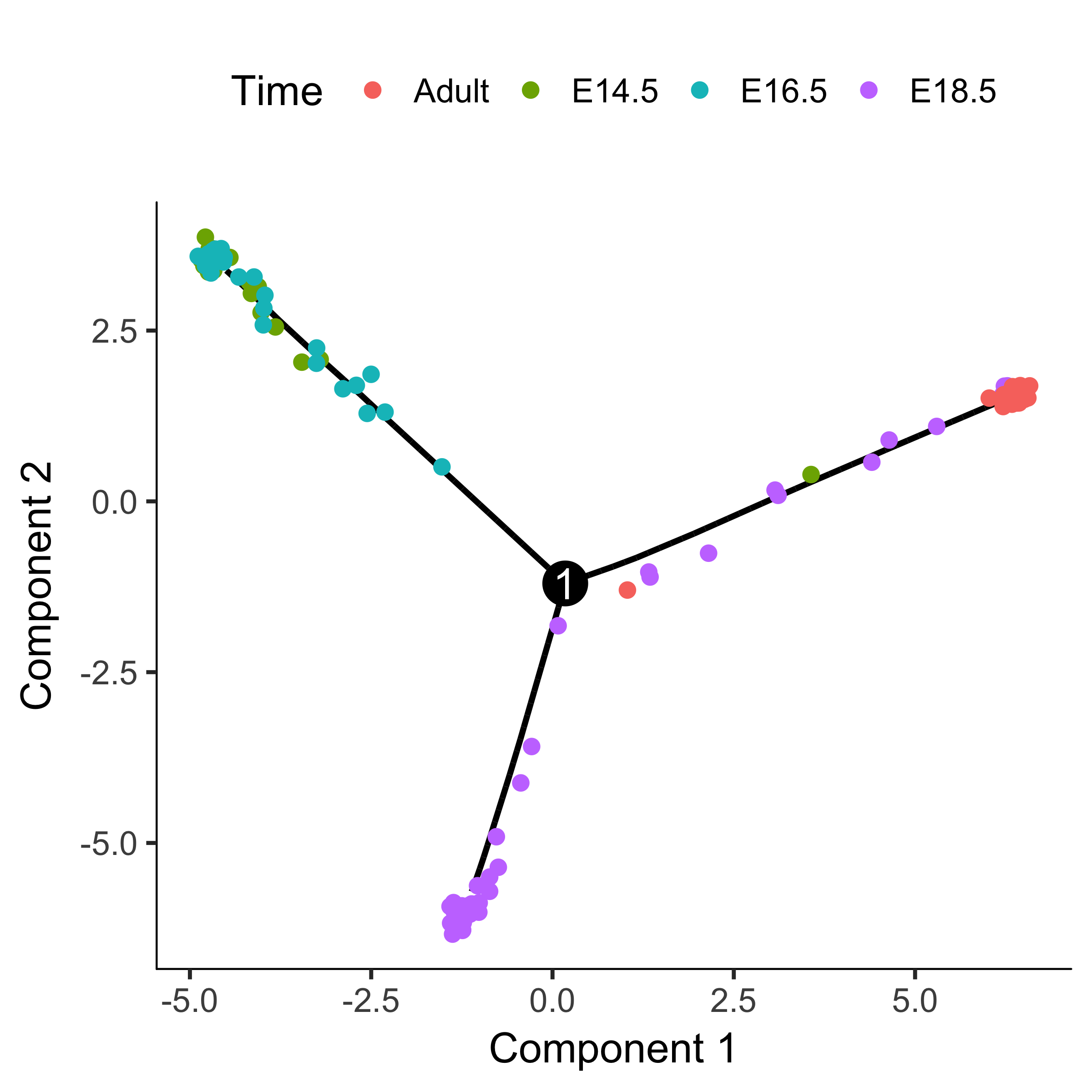
BEAM takes as input a CellDataSet that's been ordered with orderCells and the name of a branch point in the trajectory.
It returns a table of significance scores for each gene.
Genes that score significant are said to be branch-dependent in their expression.
BEAM_res <- BEAM(lung, branch_point = 1, cores = 1)
BEAM_res <- BEAM_res[order(BEAM_res$qval),]
BEAM_res <- BEAM_res[,c("gene_short_name", "pval", "qval")]
You can visualize changes for all the genes that are significantly branch dependent using a special type of heatmap. This heatmap shows changes in both lineages at the same time. It also requires that you choose a branch point to inspect. Columns are points in pseudotime, rows are genes, and the beginning of pseudotime is in the middle of the heatmap. As you read from the middle of the heatmap to the right, you are following one lineage through pseudotime. As you read left, the other. The genes are clustered hierarchically, so you can visualize modules of genes that have similar lineage-dependent expression patterns.
plot_genes_branched_heatmap(lung[row.names(subset(BEAM_res,
                                          qval < 1e-4)),],
                                          branch_point = 1,
                                          num_clusters = 4,
                                          cores = 1,
                                          use_gene_short_name = T,
                                          show_rownames = T)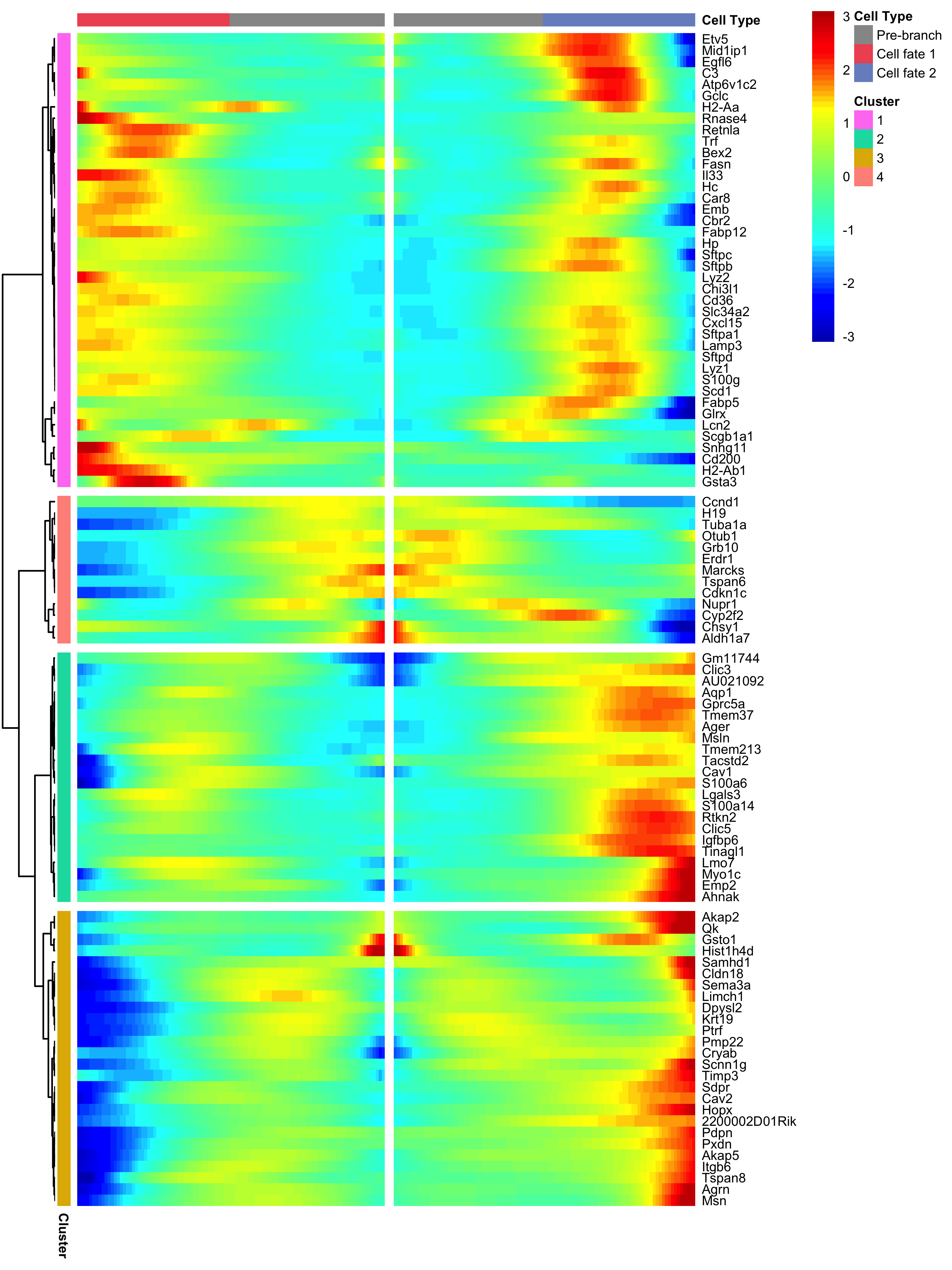
We can plot a couple of these genes, such as Pdpn and Sftpb (both known markers of fate in this system), using the plot_genes_branched_pseudotime function, which works a lot like the plot_genes_in_pseudotime function, except it shows two kinetic trends, one for each lineage, instead of one.
We also show Ccnd2, a cell cycle gene, which is downregulated in both branches and is not signficant by the BEAM test.
lung_genes <- row.names(subset(fData(lung),
          gene_short_name %in% c("Ccnd2", "Sftpb", "Pdpn")))
plot_genes_branched_pseudotime(lung[lung_genes,],
                       branch_point = 1,
                       color_by = "Time",
                       ncol = 1)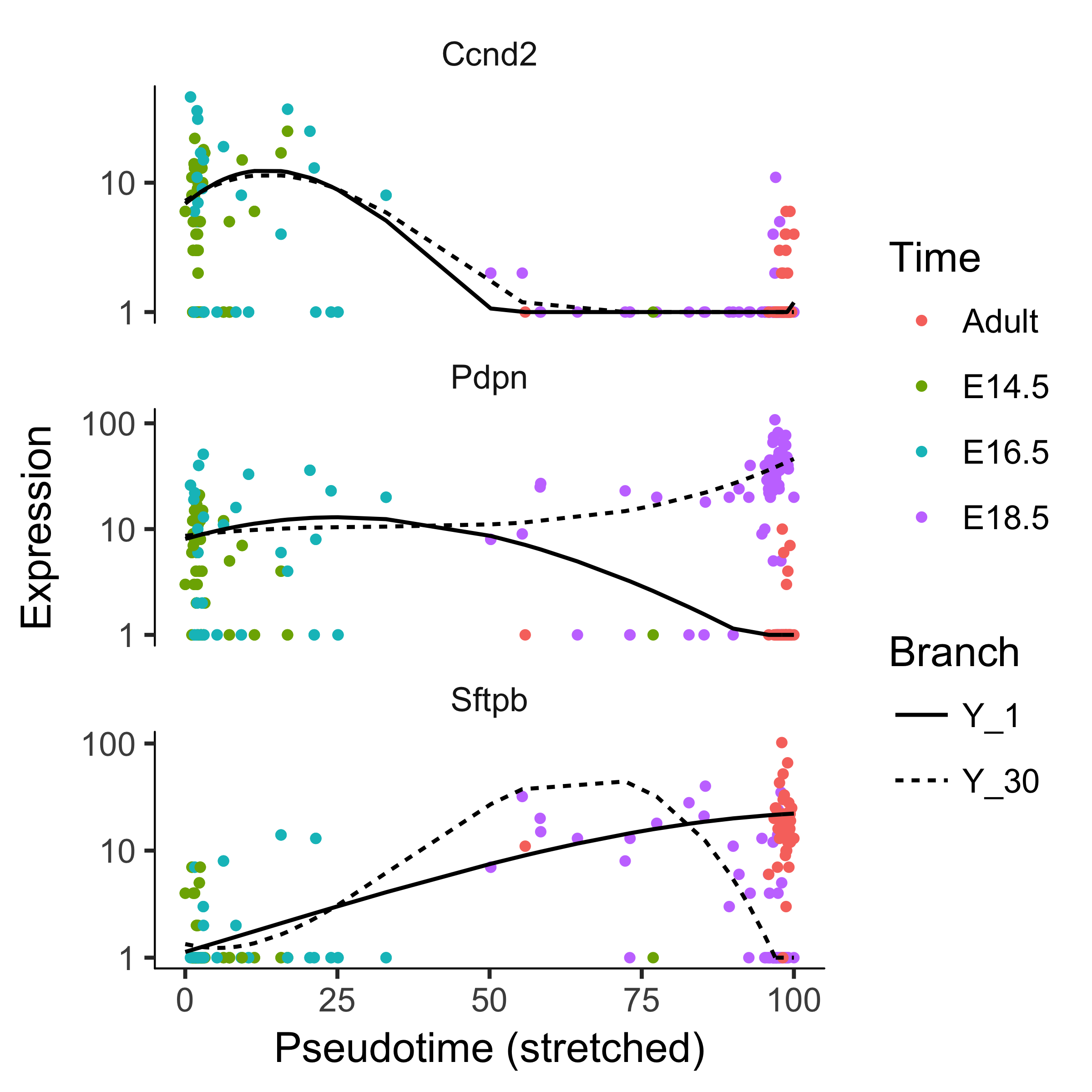
The plot_clusters function returns a ggplot2 object showing the shapes of the expression patterns followed by the 100 genes we've picked out.
The topographic lines highlight the distributions of the kinetic patterns relative to the overall trend lines, shown in red.
Appendices
Computing Expression Values for Single Cells
To use Monocle, you must first compute the expression of each gene in each cell for your experiment. There are a number of ways to do this for RNA-Seq. We recommend using Cufflinks, but you could also use RSEM, eXpress, Sailfish, or another tool for estimating gene and transcript expression levels from aligned reads. Here, we'll show a simplified workflow for using TopHat and Cufflinks to estimate expression. You can read more about how to use TopHat and Cufflinks to calculate expression here.
To estimate gene and transcript expression levels for single-cell RNA-Seq using
TopHat and
Cufflinks, you must have a file of RNA-Seq
reads for each cell you captured. If you performed paired-end RNA-Seq, you
should have two files for each cell. Depending on how the base calling was
performed, the naming conventions for these files may differ. In the examples
below, we assume that each file follows the format:
CELL_TXX_YYY.RZ.fastq.gz
Where XX is the time point at which the cell was collected in our experiment, YY is the well of the 96-well plate used during library prep, and Z is either 1 or 2 depending on whether we are looking at the left mate or the right mate in a paired end sequencing run. So CELL_T24_A01.R1.fastq.gz means we are looking at the left mate file for a cell collected 24 hours into our experiment and which was prepped in well A01 of the 24-hour capture plate.
Aligning reads to the genome with TopHat
We begin by aligning each cell's reads separately, so we will have one BAM file
for each cell. The commands below show how to run each cell's reads through
TopHat. These alignment commands can take a while, but they can be run in
parallel if you have access to a compute cluster. If so, contact your cluster
administrator for more information on how to run TopHat in a cluster
environment.
tophat -o CELL_T24_A01_thout -G GENCODE.gtf bowtie-hg19-idx CELL_T24_
    A01.R1.fastq.gz CELL_T24_A01.R2.fastq.gz
tophat -o CELL_T24_A02_thout -G GENCODE.gtf bowtie-hg19-idx CELL_T24_
    A02.R1.fastq.gz CELL_T24_A02.R2.fastq.gz
tophat -o CELL_T24_A03_thout -G GENCODE.gtf bowtie-hg19-idx CELL_T24_
    A03.R1.fastq.gz CELL_T24_A03.R2.fastq.gz
The commands above show how to align the reads for each of three cells in the experiment. You will need to run a similar command for each cell you wish to include in your analysis. These TopHat alignment commands are simplified for brevity - there are options to control the number of CPUs used by TopHat and otherwise control how TopHat aligns reads that you may want to explore on the TopHat manual. The key components of the above commands are:
- The
-ooption, which sets the directory in which each cell's output will be written. - The gene annotation file, specified with -G, which tells TopHat where to look for splice junctions.
- The Bowtie index for genome of your organism, in this case build hg19 of the human genome.
- The read files for each cell as mentioned above.
When the commands finish, there will be a BAM file in each cell's TopHat output
directory. For example, CELL_T24_A01_thout/accepted_hits.bam will contain the
alignments for cell T24_A01.
Computing gene expression using Cufflinks
Now, we will use Cufflinks to estimate gene expression levels for each cell in your study.
cuffquant -o CELL_T24_A01_cuffquant_out GENCODE.gtf
    CELL_T24_A01_thout/accepted_hits.bam
cuffquant -o CELL_T24_A02_cuffquant_out GENCODE.gtf
    CELL_T24_A02_thout/accepted_hits.bam
cuffquant -o CELL_T24_A03_cuffquant_out GENCODE.gtf
    CELL_T24_A03_thout/accepted_hits.bam
The commands above show how to convert aligned reads for each cell into gene expression values for that cell. You will need to run a similar command for each cell you wish to include in your analysis. These commands are simplified for brevity - there are options to control the number of CPUs used by the cuffquant utility and otherwise control how cuffquant estimates expression that you may want to explore on the [Cufflinks](http://cufflinks.cbcb.umd.edu/) manual. The key components of the above commands are:
- The -o option, which sets the directory in which each cell's output will be written.
- The gene annotation file, which tells cuffquant what the gene structures are in the genome.
- The BAM file containing the aligned reads.
Next, you will need to merge the expression estimates into a single table for
use with Monocle. You can do this with the following command:
cuffnorm --use-sample-sheet -o sc_expr_out GENCODE.gtf
    sample_sheet.txt
The option --use-sample-sheet tells cuffnorm that it should look in the file
sample_sheet.txt for the expression files, to make the above command simpler. If
you choose not to use a sample sheet, you will need to specify the expression
files on the command line directly. The sample sheet is a tab-delimited file
that looks like this:
sample_name                                   group
CELL_T24_A01_cuffquant_out/abundances.cxb     T24_A01
CELL_T24_A02_cuffquant_out/abundances.cxb     T24_A02
CELL_T24_A03_cuffquant_out/abundances.cxb     T24_A03
Now, you are ready to load the expression data into Monocle and start analyzing your experiment.
Major updates in Monocle 2
Monocle 2 is a near-complete re-write of Monocle 1. Monocle 2 is geared towards larger, more complex single-cell RNA-Seq experiments than those possible at the time Monocle 1 was written. It's also redesigned to support analysis of mRNA counts, which were hard to estimate experimentally in early versions of single-cell RNA-Seq. Now, with spike controls or UMIs, gene expression can be measured in mRNA counts. Analysis of these counts is typically easier and more accurate than relative expression values, and we encourage all users to adopt an mRNA-count centered workflow. Numerous Monocle functions have been re-written to take advantage of the nicer statistical properties of mRNA counts. For example, we adopt the dispersion modeling and variance-stabilization techniques introduced by DESeq [6] during differential analysis, dimensionality reduction, and other steps.
Trajectory reconstruction in Monocle 2 is vastly more robust, faster, and more powerful than in Monocle 1. Monocle 2 uses an advanced nonlinear reconstruction algorithm called DDRTree [7], described below in the section Theory Behind Monocle . This algorithm can expose branches that are hard to see with the less powerful linear technique used in Monocle 1. The algorithm is also far less sensitive to outliers, so careful QC and selection of high quality cells is less critical. Finally, DDRTree is much more robust in that it reports qualititatively similar trajectories more consistently when you vary the number of cells in the experiment. Although which genes are included in the ordering still greatly impact the trajectory, varying them also produces more qualititatively consistent trajectories than the previous linear technique.
Because Monocle 2 is so much better at finding branches, it also includes some additional tools to help you interpret them. Branch expression analysis modeling (BEAM) is a new test for analyzing specific branch points [8]. BEAM reports branch-dependent genes, and Monocle 2 includes some new visualization functions to help you inspect these genes. Overall, we find that branching is pervasive in diverse biological processes, and thus we expect BEAM will be very useful to those analyzing single-cell RNA-Seq data in many settings.
Monocle 2 also includes functionality that is inspired by other packages that weren't available when Monocle 1 was written. For example, much of Monocle 2's clustering strategy is similar to Seurat [9] from Rahul Satija's lab.
A manuscript describing Monocle 2 and the general stragegy of using reversed graph embedding for single-cell trajectory analysis is available on the bioRxiv [10].
Theory Behind Monocle
dpFeature: Selecting features from dense cell clusters
Appling algorithms like t-SNE to cells transiting through a continuous process like cell differentiation often groups the cells into clusters that do not necessarily reflect their progression through the process. Nevertheless, the genes that are differentially expressed by cells the clusters are often highly informative markers of each cell's progress through the trajectory. That is, clustering algorithms like t-SNE can find often genes that vary over the trajectory, but not the trajectory itself. We designed a simple procedure to identify these genes for use in trajectory reconstruction.
The dpFeature procedure works as follows. First, dpFeature excludes genes that only expressed in a very small percentage of cells (by default, 5%). Second, dpFeature performs PCA on the remaining genes in order to identify the principal components that explain a substantial amount of variance in the data. These top PCs are then used to initialize t-SNE, which projects the cells into two-dimensional t-SNE space. Next, dpFeature uses a recently developed clustering algorithm, called "density peak" clustering [4] to cluster the cells in the two-dimensional t-SNE space. The density peak clustering algorithm calculates each cell's local density (Ρ) and its distance (Δ) to another cell with higher density. The Ρ and Δ values for each cell can be plotted in a so-called "decision plot" in order to select thresholds that define "peaks" in the t-SNE space. Cells with high local density that are far away from other cells with high local density correspond to the density peaks. These density peaks nucleate clusters: all other cells will be associated with the nearest density peak cell. Finally, we identify genes that differ between the clusters by performing a likelihood ratio test between using a generalized linear model that knows the cluster to which each cell is assigned and a model that doesn't. We then select (by default) the top 1,000 significantly differentially expressed genes as the ordering genes for the trajectory reconstruction.
Reversed graph embedding
Single-cell expression datasets are some of the largest and most complex encountered in genomics. Even the smallest single-cell RNA-Seq experiments sample hundreds of cells, measuring the expression level of the more than 20,000 genes in each cell. Visualizing these datasets, identifying cells of different types, and comparing them to one another all pose major bioinformatics challenges.
Manifold learning is a common strategy for dealing with complex, high-dimensional data. The premise of this approach is simple: the data may reside in a very high-dimensional space, but the intrinsic structure of the dataset is much simpler. Moreover, the data are not random - they are generated by a process that can be understood by inspecting the global structure of the dataset. For example, a single single-cell RNA-Seq experiment may reside in 20,000 dimensions, but the cells might all lie on or "near" a curve embedded within a much lower dimensional space. For example, we might expect that cells in different phases of the cell cycle be distributed along a closed loop. Indeed a recent large-scale single-cell RNA-Seq study found exactly that [11].
Manifold learning often involves dimensionality reduction techniques as a first step. Conventional dimensionality reduction approaches (for example, PCA, ICA, Isomap, LLE, etc.) are limited in their ability to explictly recover the intrinisic structure from the data.
Monocle 2 uses a technique called reversed graph embedding [10, 12] to learn the structure of the manifold that describes a single-cell experiment. It simultaneously:
- Reduces high dimensional expression data into a lower dimension space.
- Learns an explicit, smooth manifold that generates the data.
- Assigns each cell to its position on that manifold
Together, these tasks allow Monocle 2 to order cells in pseudotime in an entirely unsupervised, data-driven way. Importantly, Monocle 2 learns manifolds that are trees without needing any a priori information about the structure of the tree. Users do not need to provide Monocle 2 with constraints on the number of branches, etc. These are learned from the data. This allows Monocle 2 to to discriminate between linear and branched trajectories automatically. To our knowledge, Monocle 2 is the first trajectory reconstruction algorithm to learn smooth tree-like manifolds without needing to know its high-level structure ahead of time.
Reversed graph embedding simultaneously learns a principal graph that approximates the manifold, as well as a function that maps points on the graph (which is embedded in low dimensions) back to the original high dimensional space. Reversed graph embedding aims to learn both a set of latent points $$ \mathcal{Z} = \{\mathbf{z}_1, ..., \mathbf{z}_M\}$$corresponding to the input data that reside in the low-dimensional space along with a graph $\mathcal{G}$ that connects them. This graph approximates the manifold. In order to map points on the manifold back to the original high-dimensional input space, we also need to learn a function $f_{\mathcal{G}}$.
Learning a good reversed graph embedding can be described as an optimization problem that joint captures the positions of the latent points $\mathbf{z}$, the graph $\mathcal{G}$, and the function $f_\mathcal{G}$.
To learn the positions of the latent points $\mathbf{z}$, we must optimize: \begin{equation} \mathop{min}_{f_g \in \mathcal{F}} \mathop{min}_{\{\mathbf{z}_1, ..., \mathbf{z}_M\}} \sum_{i = 1}^N ||\mathbf{x}_i - f_g (\mathbf{z}_i)||^2 \end{equation}
Given a set of latent point coordinates, the optimization of graph inference can be represented as: \begin{equation} \label{eq:mintree} \mathop{min}_{f_\mathcal{G} \in \mathcal{F}} \mathop{min}_{\{\mathbf{z}_1, ..., \mathbf{z}_M\}} \sum_{(V_i, V_j) \in \mathcal{E}} b_{i,j}||f_g(\mathbf{z}_i) - f_g(\mathbf{z}_j)||^2 \end{equation}
where $\mathcal{X} = \{ \mathbf{x}_1, ..., \mathbf{x}_N\}$ are the original single-cell expression profiles. The $V_i$ are the the vertices of the undirected graph $\mathcal{G} = (\mathcal{V}, \mathcal{E})$. The weights for the edge in $\mathcal{E}$ are encoded as $b_{ij}$.
The first optimization problem aims to position the latent points such that their image under $f_\mathcal{G}$ (that is, their corresponding positions in the high-dimensional space) will be "close" to the input data. The second optimization aims to keep latent points that are close to one another in the low dimensional space close to one another in the high dimensional space as well. These two goals must be balanced against one another. Reversed graph embedding achieves this through the parameter $\lambda$ \begin{equation} \mathop{min}_{\mathcal{G} \in \hat{\mathcal{G}}_b}\mathop{min}_{f_g \in \mathcal{F}} \mathop{min}_{\{\mathbf{z}_1, ..., \mathbf{z}_M\}} \sum_{i = 1}^N ||\mathbf{x}_i - f_g (\mathbf{z}_i)||^2 + \frac{\lambda}{2} \sum_{(V_i, V_j) \in \mathcal{E}} b_{i,j}||f_g(\mathbf{z}_i) - f_g(\mathbf{z}_j)||^2 \end{equation}
Reversed graph embedding requires a feasible set $\hat{\mathcal{G}}_b$ of graphs and a mapping function $f_\mathcal{G}$. In practice, implementing reversed graph embedding requires that we place some constraints on $\hat{\mathcal{G}}_b$ and $f_\mathcal{G}$. As work on reversed graph embedding continues, we anticipate that more general schemes that consider a wider range of feasible graphs and mapping functions will become available. Monocle users should expect more general reversed graph embedding schemes in future versions.
Mao et al initially described two specific ways to implement the general framework of reversed graph embedding. Both are briefly summarized below. See the original paper on DDRTree for more details. Monocle 2 uses the second scheme, but can easily be run in a mode that corresponds to the first.
DRTree: Dimensionality Reduction via Learning a Tree
The first scheme, called "DRTree" described by Mao et al learns principal graphs that are undirected trees, with one node per input data point, along with a linear function $f_\mathcal{G}$. Because the algorithm restricts the feasible set to trees, optimization problem 2 is solved by simply finding the minimum spanning tree. This can be solved quickly via Kruskal's algoritm. DRTree uses a linear projection model $f_\mathcal{G} (\mathbf{z}) = \mathbf{Wz}$ as the mapping function. The scheme optimizes: \begin{equation} \mathop{min}_{\mathbf{W}, \mathbf{Z}, \mathbf{B}} \sum_{i = 1}^N ||\mathbf{x}_i - \mathbf{W}\mathbf{z}_i||^2 + \frac{\lambda}{2} \sum_{i,j}b_{i,j}||\mathbf{W} \mathbf{z}_i - \mathbf{W} \mathbf{z}_j||^2 \end{equation}
where $\mathbf{W} = [\mathbf{w}_1, ..., \mathbf{w}_d] \in \mathcal{R}^{D \times d}$ is an orthogonal set of $d$ linear basis vectors. Because several key steps of the above optimization can be solved analytically, and because the two terms can be minimized in an alternating fashion, solving it is generally very fast. However, for large input datasets, the graph can become complex, and so DRTree can run into scalability problems.
DDRTree: discriminative dimensionality reduction via learning a tree
To overcome problems posed by large complex input datasets, Mao et al
proposed a second scheme, "DDRTree". that Monocle 2 uses instead of DRTree. Recall that the
graph in DRTree contains one node per input data point. To avoid long computations and large memory footprints that come with DRTree, the second scheme
learns a graph on a second, smaller set of latent points $\{\mathbf{y}_k\}_{k = 1}^K$.
These points are treated by the algorithm as the centers of $\{\mathbf{z}_i\}^N_{i = 1}$.
The number of these points is controlled through the ncenter argument
to reduceDimension() in Monocle 2. Using this algorithm drastically
speeds up the computations in reduceDimension(), and also serves
to regularize the manifold, often producing cleaner, more accurate single-cell
trajectories.
The DDRTree scheme works via the following optimization: \begin{equation}\label{eq:DDRTree_opt} \mathop{min}_{\mathbf{W}, \mathbf{Z}, \mathbf{B}, \mathbf{Y}, \mathbf{R}} \sum_{i = 1}^N ||\mathbf{x}_i - \mathbf{W} \mathbf{z}_i||^2 + \frac{\lambda}{2} \sum_{k, k'}b_{k, k'}||\mathbf{W} \mathbf{y}_k - \mathbf{W} \mathbf{y}_k'||^2 + \gamma\Big[\sum_{k = 1}^K \sum_{i = 1}^N r_{i, k} ||\mathbf{z}_i - \mathbf{y}_k||^2 + \sigma \Omega (\mathbf{R})\Big] \end{equation}
The optimization is constrained such that $\mathbf{W}^T \mathbf{W} = \mathbf{I}, \sum_{k = 1}^K r_{i, k} = 1, r_{i, k} \leq 0, \forall i, \forall k$. The matrix $\mathbf{R} \in \mathcal{R}^{N \times N}$ is used to regularize the graph, through the negative entropy regularization $\Omega(\mathbf{R}) = \sum_{i = 1}^N \sum_{k = 1}^k r_{i, k} \log \ r_{i, k}$. In effect, DDRTree uses the latent points $\{\mathbf{y}_k\}_{k = 1}^K$ as the centers of $K$ clusters. That is, the algorithm acts as soft K-means clustering on the points $\{\mathbf{z}_i\}^N_{i = 1}$, and jointly learns a graph on the $K$ cluster centers. The matrix $\mathbf{R}$ transforms the hard assignments used in K-means into soft assignments with $\sigma > 0$ as a regularization parameter.
Problem 5 again contains a number of analytical steps, and can be solved by alternating between the terms. Moreover, because some of the more expensive numerical operations involve matrices that are $K$ dimensional (instead of $N$ dimensional), they have complexity that is invariant of the size of the input data.
Our accessory package DDRTree implements the DDRTree algorithm using a number of key performance optimizations. Monocle 2 calls DDRTree to learn the core manifold describing a CellDataSet, and then computes pseudotime coordinates and branch assignments using this manifold. Monocle also uses the manifold in downstream analysis steps such as BEAM. A manuscript describing the general stragegy of using reversed graph embedding for single-cell trajectory analysis is available on bioRxiv [10].
Census
In [8], we introduced Census, a normalization method to convert of single-cell mRNA transcript to relative transcript counts. Using relative transcript counts (or spike-in derived counts or UMI counts if available) with the negative binomial distribution can dramatically improve the differential expression test compared to using the negative binomial with read counts or the Tobit with TPM/FPKM values. Census aims to convert relative abundances $X_{ij}$ into lysate transcript counts $Y_{ij}$. Without loss of generality, we consider relative abundances is on the TPM scale, and assume that a gene's TPM value is proportional to the relative frequencies of its mRNA within the total pool of mRNA in a given cell's lysate, i.e., $TPM_{ij} \propto \frac{Y_{ij}}{\sum_{j = 1}Y_{ij}}$. The generative model discussed in Qiu et al. predicts that when only a minority of the transcripts in a cell is captured in the library, signal from most detectably expressed genes will originate from a single mRNA. Because the number of sequencing reads per transcript is proportionate to molecular frequency after normalizing for length (i.e. TPM or FPKM), all such genes in a given cell should have similar TPM values.
Census works by first identifying the (log-transformed) TPM value in each cell $i$, written as $x_i^*$, that corresponds to genes from which signal originates from a single transcript. Because our generative model predicts that these most detectable genes should fall into this category, we simply estimate $x_i^*$ as the mode of the log-transformed TPM distribution for cell $i$. This mode is obtained by log-transforming the TPM values, performing a Gaussian kernel density estimation and then identifying the peak of the distribution. Given the TPM value for a single transcript in cell $i$, it is straightforward to convert all relative abundances to their lysate transcript counts. The total number of mRNAs captured for cell $i$ can be estimated as:
\begin{equation} M_i = \frac{1}{\theta} \cdot \frac{n_i}{\frac{1}{T} \int_{\epsilon}^{X_i^*}X_{i,j}dX} \end{equation} where (Ε) is a TPM value below which no mRNA is believed to be present (by default, $0.1$), $n_i$ is the number of genes with TPM values in the interval ($\epsilon, x_i^*$) and $T$ is the sum of TPM values of all expressed genes in a single cell. That is, we could estimate the total mRNA counts as the total number of single-mRNA genes divided by their combined expression relative to all genes, as illustrated in Figure 1A of [8]. However, cDNA and PCR amplification steps during library prep can lead to superlinear growth in the relative abundance of a transcript as a function of copy number. In practice, the above formula often over-estimates total mRNAs in the lysate. To alleviate this issue, we used an alternative formula in Census: \begin{equation} %\begin{align*}\textsc{} M_i = \frac{1}{\theta} \cdot \frac{n_i}{F_{X_i}(X_i^*) - F_{X_i}(\epsilon)} = \frac{1}{\theta} \cdot \frac{n_i}{F_{X_i}(X_i^*)}\quad\quad\quad\quad (x \geq \epsilon) %\end{align*} \end{equation} where $F_{X_i}$ represents the cumulative distribution function for the TPM values of genes expressed above (Ε) for cell $i$. Effectively, this simple approach estimates the pre-amplification cDNA count as the number of genes expressed above (Ε). Although this is necessarily an underestimate, in practice it is typically close to the true total (as shown in Figure 1c in [8]), since a large fraction of genes are expressed at 1 cDNA copy. Note that we also scale the cDNA count by 1/(Θ) to yield an estimate for the number of mRNAs that were in the cell's lysate, including those that were not actually captured. This scaling step is performed mainly to facilitate comparison with spike-in derived estimates. While we do not know the capture rate (Θ) a priori, it is a highly protocol-dependent quantity that appears to have little dependence on cell type or state. In the original study [8], we assume a value of 0.25, which is close to the lung and neuron experiments of Truetlein et al. With an estimate of the total lysate mRNAs Mi in cell i, we simply rescale its TPM values into mRNA counts for each gene: \begin{equation} \hat{Y}_{ij} = X_{ij} \cdot \frac{M_i} {10^6} \end{equation}For more details about Census, including a generative model of the single-cell RNA-seq process, and some discussion of Census's limitations, please see the original study [8]. Importantly, Census cannot control for non-linear amplification, and should therefore be considered as a simple but effective way to normalize relative expression levels so that they work better with the negative binomial distribution. Census counts should not be treated as absolute transcript counts.
BEAM
Monocle 2 assigns each cell a pseudotime value and a "State" encoding the segment of the trajectory it resides upon based on a trajectory learning algorithm (See below). In Monocle 2, we develop BEAM to test for branch-dependent gene expression by formulating the problem as a contrast between two negative binomial GLMs. The null model \begin{equation} expression \sim sm.ns(Pseudotime) \end{equation} for the test assumes the gene being tested is not a branch specific gene, whereas the alternative model: \begin{equation} expression \sim sm.ns(Pseudotime) + Branch + sm.ns(Pseudotime) : Branch \end{equation} assumes that the gene is a branch specific gene where : represents an interaction term between branch and transformed pseudotime. Each model includes a natural spline (here with three degrees of freedom) describing smooth changes in mean expression as a function of pseudotime. The null model fits only a single curve, whereas the alternative will fit a distinct curve for each branch. Our current implementation of Monocle 2 relies on VGAM's "smart" spline fitting functionality, hence the use of the sm.ns() function instead of the more widely used ns() function from the splines package in R. Likelihood ratio testing was performed with the VGAM lrtest() function, similar to Monocle's other differential expression tests. A significant branch-dependent genes means that the gene has distinct expression dynamics along each branch, with smoothed curves that have different shapes.To fit the full model, each cell must be assigned to the appropriate branch, which is coded through the factor "Branch" in the above model formula. Monocle's function for testing branch dependence accepts an argument specifying which branches are to be compared. These arguments are specified using the 'State' attribute assigned by Monocle during trajectory reconstructions. For example, in our analysis of the Truetlein et al data, Monocle 2 reconstructed a trajectory with two branches LAT1, LAT2 for AT1 and AT2 lineages, respectively), and three states (SBP, LAT1, LAT2 for progenitor, AT1, or AT2 cells). The user specifies that he or she wants to compare LAT1 and LAT2 by providing SAT1 and SAT2 as arguments to the function. Alternatively, the user can specify a branch point leading to the two states. Monocle then assigns all the cells with state SAT1 to branch LAT1 and similarly for the AT2 cells. However, the cells with SBP must be members of both branches, because they are on the path from each branch back to the root of the tree. In order to ensure the independence of data points required for the LRT as well as the robustness and stability of our algorithm, we implemented a strategy to partition the progenitor cells into two groups, with each branch receiving a group. The groups are computed by simply ranking the progenitor cells by pseudotime and assigning the odd-numbered cells to one group and the even numbered cells to the other. We assign the first progenitor to both branches to ensure they start at the same time which is required for spline fitting involved in the test.
In order to facilitate downstream branch kinetic curve clusterin as well as branch time point detection. In the current implmentation of monocle 2, we duplicate the progenitor cells and assign it to both lineage before spline fitting. The branch plots in the section Analyzing Branches in Single-Cell Trajectories use this method.Branch time point detection
The branching time point for each gene can be quantified by fitting a separate spline curves for each branch from all the progenitor to each cell fate. To robustly detect the pseudotime point (tbetai) when a gene i with a branching expression pattern starts to diverge between two cell fates L1, L2, we developed the branch time point detection algorithm. The algorithm starts from the end of stretched pseudotime (pseudotime $t = 10$ , see the supplementary note 1 for details) to calculate the divergence ($D_i(t = 100) = x_{L_1}(t = 100) - x_{L_2}(t = 100)$) of gene i's expression ($x_{L_1}(t = 100), x_{L_2}(t = 100)$) between two cell fates, $L_1, L_2$ , (for a branching gene, the divergence at this moment should be large if not the largest across pseudotime). It then moves backwards to find the latest intersection point between two fitted spline curves, which corresponds to the time when the gene starts to diverge between two branches. To add further flexibility, the algorithm moves forward to find the time point when the gene expression diverges up to a user controllable threshold ($\epsilon$), or $D_i(t) \geq \epsilon (t)$, and defines this time point as the branch time point, $t_{\beta}^i$ , for that particular gene i.Citation
If you use Monocle to analyze your experiments, please cite:citation("monocle")
## Cole Trapnell and Davide Cacchiarelli et al (2014): The dynamics
## and regulators of cell fate decisions are revealed by
## pseudo-temporal ordering of single cells. Nature Biotechnology
##
## Xiaojie Qiu, Andrew Hill, Cole Trapnell et al (2017):
## Single-cell mRNA quantification and differential analysis with
## Census. Nature Methods
##
## Xiaojie Qiu, Cole Trapnell et al (2017): Reverse graph embedding
## resolves complex single-cell developmental trajectories. BioRxiv
##
## To see these entries in BibTeX format, use 'print(<citation>,
## bibtex=TRUE)', 'toBibtex(.)', or set
## 'options(citation.bibtex.max= 999)'.Acknowledgements
Monocle was originally built by Cole Trapnell and Davide Cacchiarelli, with substantial design input John Rinn and Tarjei Mikkelsen. We are grateful to Sharif Bordbar, Chris Zhu, Amy Wagers and the Broad RNAi platform for technical assistance, and Magali Soumillon for helpful discussions. Cole Trapnell is a Damon Runyon Postdoctoral Fellow. Davide Cacchiarelli is a Human Frontier Science Program Fellow. Cacchiarelli and Mikkelsen were supported by the Harvard Stem Cell Institute. John Rinn is the Alvin and Esta Star Associate Professor. This work was supported by NIH grants 1DP2OD00667, P01GM099117, and P50HG006193-01. This work was also supported in part by the Single Cell Genomics initiative, a collaboration between the Broad Institute and Fluidigm Inc. Monocle 2 was developed by Cole Trapnell's lab. Significant portions were written by Xiaojie Qiu. The work was supported by NIH grant 1DP2HD088158 as well as an Alfred P. Sloan Foundation Research Fellowship. This vignette was created from Wolfgang Huber's Bioconductor vignette style document, and patterned after the vignette for DESeq, by Simon Anders and Wolfgang Huber.References
[1] Cole Trapnell, Davide Cacchiarelli, Jonna Grimsby, Prapti Pokharel, Shuqiang Li, Michael Morse, Niall J. Lennon, Kenneth J. Livak, Tarjei S. Mikkelsen, and John L. Rinn. The dynamics and regulators of cell fate decisions are revealed by pseudotemporal ordering of single cells. Nature Biotechnology, 2014.
[2] Cole Trapnell, Adam Roberts, Loyal Goff, Geo Pertea, Daehwan Kim, David R Kelley, Harold Pimentel, Steven L Salzberg, John L Rinn, and Lior Pachter. Differential gene and transcript expression analysis of RNA-seq experiments with TopHat and Cufflinks. Nature Protocols, 7(3):562–578, March 2012.
[3] Laurens van der Maaten and Geoffrey Hinton. Visualizing data using t-SNE. J. Mach. Learn. Res., 9(Nov):2579– 2605, 2008.
[4] Alex Rodriguez. Alessandro Laio. Clustering by fast search and find of density peaks. Science, 344:1492–1496, 2014.
[5] Hadley Wickham. ggplot2: Elegant Graphics for Data Analysis. Springer-Verlag New York, 2009.
[6] Simon Anders and Wolfgang Huber. Differential expression analysis for sequence count data. Genome Biol., 11(10):R106, 2010.
[7] Qi Mao, Li Wang, Steve Goodison, and Yijun Sun. Dimensionality reduction via graph structure learning. In Proceedings of the 21th ACM SIGKDD International Conference on Knowledge Discovery and Data Mining, pages 765–774. ACM, 2015.
[8] X Qiu, A Hill, J Packer, D Lin, YA Ma, and C Trapnell. Single-cell mrna quantification and differential analysis with census. Nature methods, 2017.
[9] Rahul Satija, Jeffrey A Farrell, David Gennert, Alexander F Schier, and Aviv Regev. Spatial reconstruction of single-cell gene expression data. Nat. Biotechnol., 33(5):495–502, May 2015.
[10] Xiaojie Qiu, Qi Mao, Ying Tang, Li Wang, Raghav Chawla, Hannah Pliner, and Cole Trapnell. Reversed graph embedding resolves complex single-cell developmental trajectories. 21 February 2017.
[11] Evan Z Macosko, Anindita Basu, Rahul Satija, James Nemesh, Karthik Shekhar, Melissa Goldman, Itay Tirosh, Allison R Bialas, Nolan Kamitaki, Emily M Martersteck, John J Trombetta, David A Weitz, Joshua R Sanes, Alex K Shalek, Aviv Regev, and Steven A McCarroll. Highly parallel genome-wide expression profiling of individual cells using nanoliter droplets. Cell, 161(5):1202–1214, 2015.
[12] Qi Mao, Li Wang, Ivor Tsang, and Yijun Sun. Principal graph and structure learning based on reversed graph embedding . IEEE Trans. Pattern Anal. Mach. Intell., 5 December 2016.
[13] Cabili, Moran N. et al. Integrative Annotation of Human Large Intergenic Noncoding RNAs Reveals Global Properties and Specific Subclasses. Genes & Development 25.18 (2011): 1915–1927. PMC. Web. 21 June 2017.