Cicero for Monocle/Monocle 2
Abstract
Cicero is an R package that provides tools for analyzing single-cell chromatin accessibility experiments. The main function of Cicero is to use single-cell chromatin accessibility data to predict cis-regulatory interactions (such as those between enhancers and promoters) in the genome by examining co-accessibility. In addition, Cicero extends Monocle to allow clustering, ordering, and differential accessibility analysis of single cells using chromatin accessibility. For more information about Cicero, explore our publications.
Introduction
The main purpose of Cicero is to use single-cell chromatin accessibility data to predict regions of the genome that are more likely to be in physical proximity in the nucleus. This can be used to identify putative enhancer-promoter pairs, and to get a sense of the overall stucture of the cis-architecture of a genomic region.
Because of the sparsity of single-cell data, cell must be aggregated by similarity to allow robust correction for various technical factors in the data.
Ultimately, Cicero provides a "Cicero co-accessibility" score between -1 and 1 between each pair of accessibile peaks within a user defined distance where a higher number indicates higher co-accessibility.
In addition, the Cicero package provides an extension toolkit for analyzing single-cell ATAC-seq experiments using the framework provided by Monocle. This vignette provides an overview of a single-cell ATAC-Seq analysis workflow with Cicero. For further information and more options, please see the manual pages for the Cicero R package, and our publications.
Cicero can help you perform two main types of analysis:
- Constructing and analysing cis-regulatory networks. Cicero analyzes co-accessibility to identify putative cis-regulatory interactions, and uses various techniques to visualize and analyze them.
- General single-cell chromatin accessibility analysis . Cicero also extends the software package Monocle to allow for identification of differential accessibility, clustering, visualization, and trajectory reconstruction using single-cell chromatin accessibility data.
Before we look at Cicero's functions for each of these analysis tasks, let's see how to install Cicero.
Installing Cicero
Cicero runs in the R statistical computing environment. You will need R version 3.4 or higher and Cicero 1.0.0 or higher to have access to the latest features.
Install from Bioconductor
Cicero was recently added to Bioconductor. It has been released as part of Bioconductor 3.8 and can be installed with the following code:
if (!requireNamespace("BiocManager", quietly = TRUE))
  install.packages("BiocManager")
BiocManager::install("cicero")
Install from Github
For the absolute latest updates to the Cicero package, you can install Cicero directly from the github repository using these instructions:
Cicero builds upon a package called Monocle. Before installing Cicero, first, follow these instructions to install Monocle.
In addition to Monocle, Cicero requires the following packages from Bioconductor
if (!requireNamespace("BiocManager", quietly = TRUE))
    install.packages("BiocManager")
BiocManager::install(c("Gviz", "GenomicRanges", "rtracklayer"))
You're now ready to install Cicero:
install.packages("devtools")
devtools::install_github("cole-trapnell-lab/cicero-release")
Load Cicero
After installation, test that Cicero installed correctly by opening a new R session and typing:
library(cicero)Getting help
Questions about Cicero should be posted on our Google Group. Please do not email technical questions to Cicero contributors directly.
Recommended analysis protocol
The Cicero workflow is broken up into broad steps. When there's more than one way to do a certain step, we've labeled the options as follows:
| Required | You need to do this. |
| Recommended | Of the ways you could do this, we recommend you try this one first. |
| Alternative | Of the ways you could do this, this way might work better than the one we usually recommend. |
Loading your data
The CellDataSet class
Cicero holds data in objects of the
CellDataSet (CDS) class. The class is derived from the Bioconductor ExpressionSet
class, which provides a common interface familiar to those who have analyzed microarray experiments with
Bioconductor. Monocle provides detailed documentation about how to generate an input CDS
here.
To modify the CDS object to hold chromatin accessibility rather than expression data, Cicero uses peaks as
its feature data fData rather than genes or transcripts. Specifically, many Cicero functions
require peak information in the form chr1_10390134_10391134. For example, an input fData table might look
like this:
| site_name | chromosome | bp1 | bp2 | |
|---|---|---|---|---|
| chr10_100002625_100002940 | chr10_100002625_100002940 | 10 | 100002625 | 100002940 |
| chr10_100006458_100007593 | chr10_100006458_100007593 | 10 | 100006458 | 100007593 |
| chr10_100011280_100011780 | chr10_100011280_100011780 | 10 | 100011280 | 100011780 |
| chr10_100013372_100013596 | chr10_100013372_100013596 | 10 | 100013372 | 100013596 |
| chr10_100015079_100015428 | chr10_100015079_100015428 | 10 | 100015079 | 100015428 |
Loading data from a simple sparse matrix format
The Cicero package includes a small dataset called cicero_data as an example.
data(cicero_data)
For convenience, Cicero includes a function called make_atac_cds. This function takes as input a
data.frame or a path to a file in a sparse matrix format. Specifically, this file should be a
tab-delimited text file with three columns. The first column is the peak coordinates in the form
"chr10_100013372_100013596", the second column is the cell name, and the third column is an integer that
represents the number of reads from that cell overlapping that peak. The file should not have a header line.
For example:
| chr10_100002625_100002940 | cell1 | 1 |
|---|---|---|
| chr10_100006458_100007593 | cell2 | 2 |
| chr10_100006458_100007593 | cell3 | 1 |
| chr10_100013372_100013596 | cell2 | 1 |
| chr10_100015079_100015428 | cell4 | 3 |
The output of make_atac_cds is a valid CDS object ready to be input into downstream Cicero
functions.
input_cds <- make_atac_cds(cicero_data, binarize = TRUE)make_atac_cds
| Option | Default | Notes |
|---|---|---|
binarize |
FALSE | Logical, should the count matrix be converted to binary? Because of the sparsity of single-cell data, we don't generally expect more than 1 read per cell per peak. We have found that converting a count matrix to a binary "is this site open in this cell" can ultimately give clearer results. |
Loading 10X scATAC-seq data
If your scATAC-seq data comes from the 10x Genomics platform, here is an example of creating your input CDS from the output of Cell Ranger ATAC. The output of interest will be in the folder called filtered_peak_bc_matrix.
# read in matrix data using the Matrix package
indata <- Matrix::readMM("filtered_peak_bc_matrix/matrix.mtx")
# binarize the matrix
indata@x[indata@x > 0] <- 1

# format cell info
cellinfo <- read.table("filtered_peak_bc_matrix/barcodes.tsv")
row.names(cellinfo) <- cellinfo$V1
names(cellinfo) <- "cells"

# format peak info
peakinfo <- read.table("filtered_peak_bc_matrix/peaks.bed")
names(peakinfo) <- c("chr", "bp1", "bp2")
peakinfo$site_name <- paste(peakinfo$chr, peakinfo$bp1, peakinfo$bp2, sep="_")
row.names(peakinfo) <- peakinfo$site_name

row.names(indata) <- row.names(peakinfo)
colnames(indata) <- row.names(cellinfo)

# make CDS
fd <- methods::new("AnnotatedDataFrame", data = peakinfo)
pd <- methods::new("AnnotatedDataFrame", data = cellinfo)
input_cds <-  suppressWarnings(newCellDataSet(indata,
                            phenoData = pd,
                            featureData = fd,
                            expressionFamily=VGAM::binomialff(),
                            lowerDetectionLimit=0))
input_cds@expressionFamily@vfamily <- "binomialff"
input_cds <- monocle::detectGenes(input_cds)

#Ensure there are no peaks included with zero reads
input_cds <- input_cds[Matrix::rowSums(exprs(input_cds)) != 0,]
Constructing cis-regulatory networks
Running Cicero
Create a Cicero CDS Required
Because single-cell chromatin accessibility data is extremely sparse, accurate estimation of co-accessibility scores requires us to aggregate similar cells to create more dense count data. Cicero does this using a k-nearest-neighbors approach which creates overlapping sets of cells. Cicero constructs these sets based on a reduced dimension coordinate map of cell similarity, for example, from a tSNE or DDRTree map.
You can use any dimensionality reduction method to base your aggregated CDS on. We will show you how to create two versions, tSNE and DDRTree (below). Both of these dimensionality reduction methods are available from Monocle (and loaded by Cicero).
Once you have your reduced dimension coordinate map, you can use the function make_cicero_cds to
create your aggregated CDS object. The input to make_cicero_cds is your input CDS object, and
your reduced dimension coordinate map. The reduced dimension map reduced_coordinates should be
in the form of a data.frame or a matrix where the row names match the cell IDs from
the pData table of your CDS. The columns of reduced_coordinates should be the
coordinates of the reduced dimension object, for example:
| ddrtree_coord1 | ddrtree_coord2 | |
|---|---|---|
| cell1 | -0.7084047 | -0.7232994 |
| cell2 | -4.4767964 | 0.8237284 |
| cell3 | 1.4870098 | -0.4723493 |
Here is an example of both dimensionality reduction and creation of a Cicero CDS. Using monocle as a guide,
we first find tSNE coordinates for our input_cds:
set.seed(2017)
input_cds <- detectGenes(input_cds)
input_cds <- estimateSizeFactors(input_cds)

# *** if you are using Monocle 3 alpha, you need to run the following line as well!
# NOTE: Cicero does not yet support the Monocle 3 beta release (monocle3 package). We hope
# to update soon!
#input_cds <- preprocessCDS(input_cds, norm_method = "none")
input_cds <- reduceDimension(input_cds, max_components = 2, num_dim=6,
                      reduction_method = 'tSNE', norm_method = "none")
Next, we access the tSNE coordinates from the input CDS object where they are stored by Monocle and run
make_cicero_cds:
tsne_coords <- t(reducedDimA(input_cds))
row.names(tsne_coords) <- row.names(pData(input_cds))
cicero_cds <- make_cicero_cds(input_cds, reduced_coordinates = tsne_coords)
Run Cicero Required
The main function of the Cicero package is to estimate the co-accessiblity of sites in the genome in order to predict cis-regulatory interactions. There are two ways to get this information:
run_cicero: get Cicero outputs with all defaults The functionrun_cicerowill call each of the relevant pieces of Cicero code using default values, and calculating best-estimate parameters as it goes. For most users, this will be the best place to start.- Call functions separately, for more flexibility For users wanting more flexibility in the parameters that are called, and those that want access to intermediate information, Cicero allows you to call each of the component parts separately.
Consider non-default parameters
run_cicero Recommended
The easiest way to get Cicero co-accessibility scores is to run run_cicero. To run
run_cicero, you need a cicero CDS object (created above) and a genome coordinates file, which
contains the lengths of each of the chromosomes in your organism. The human hg19 coordinates are included
with the package and can be accessed with data("human.hg19.genome"). Here is an example call,
continuing with our example data:
data("human.hg19.genome")
sample_genome <- subset(human.hg19.genome, V1 == "chr18")
conns <- run_cicero(cicero_cds, sample_genome) # Takes a few minutes to run
head(conns)| Peak1 | Peak2 | coaccess |
|---|---|---|
| chr18_10025_10225 | chr18_104385_104585 | 0.03791526 |
| chr18_10025_10225 | chr18_10603_11103 | 0.86971957 |
| chr18_10025_10225 | chr18_111867_112367 | 0.00000000 |
Call Cicero functions individually Alternative
The alternative to calling run_cicero is to run each piece of the Cicero pipeline in pieces. The
three functions that make up the Cicero pipeline are:
estimate_distance_parameter. This function calculates the distance penalty parameter based on small random windows of the genome.generate_cicero_models. This function uses the distance parameter determined above and uses graphical LASSO to calculate the co-accessibility scores of overlapping windows of the genome using a distance-based penalty.assemble_connections. This function takes as input the output ofgenerate_cicero_modelsand reconciles the overlapping models to create the final list of co-accessibility scores.
Use the manual pages in R (example: ?estimate_distance_parameter) to see all options. Key
options are detailed below:
estimate_distance_parameter
| Option | Default | Notes |
|---|---|---|
window |
500000 | The window parameter controls how large of a window (in base pairs) in the genome is used for
calculating each individual model. This parameter will control the furthest distance between sites
that are compared. This parameter must be the same as the window parameter for
generate_cicero_models. |
sample_num |
100 | This is the number of sample regions to calculate a distance parameter for. |
distance_constraint |
250000 | The distance_constraint controls the distance at which Cicero expects few meaningful
cis-regulatory contacts. estimate_distance_parameter uses this value to estimate the
distance parameter by increasing regularization until there are few contacts at a distance beyond
the distance_constraint. The distance_constraint must be
sufficiently lower than the window parameter - as a rule of thumb, set your window to be at least
1/3 larger than your distance_constraint. |
s |
0.75 | s is a constant that captures the power-law distribution of contact frequencies
between different locations in the genome as a function of their linear distance. For a complete
discussion of the various polymer models of DNA packed into the nucleus and of justifiable values
for s, we refer readers to (Dekker et al., 2013). We use a value of 0.75 by default in
Cicero, which corresponds to the “tension globule” polymer model of DNA (Sanborn et al., 2015). For
data not from humans, we recommend you read further discussion of this parameter here:
Important
Considerations for Non-Human Data. This parameter must be the same as the
s parameter for generate_cicero_models. |
generate_cicero_models
| Option | Default | Notes |
|---|---|---|
window |
500000 | The window parameter controls how large of a window (in base pairs) in the genome is used for
calculating each individual model. This parameter will control the furthest distance between sites
that are compared. This parameter must be the same as the window parameter for
estimate_distance_parameter. |
distance_parameter |
100 | The distance_parameter controls the distance-based scaling of the regularization
parameter in graphical LASSO. This parameter is generally the mean of the sample values calculated
using estimate_distance_parameter |
s |
0.75 | See above in the documentation for estimate_distance_parameter. This parameter
must be the same as the s parameter for
estimate_distance_parameter. |
assemble_connections
| Option | Default | Notes |
|---|---|---|
silent |
FALSE | Logical, whether to print summary information. |
Visualizing Cicero Connections
The Cicero package includes a general plotting function for visualizing co-accessibility called
plot_connections. This function uses the
Gviz framework for plotting
genome browser-style plots. We have adapted a function from the
Sushi R package for
mapping connections. plot_connections has many options, some detailed in the
Advanced Visualization section, but to get a
basic plot from your co-accessibility table is quite simple:
data(gene_annotation_sample)
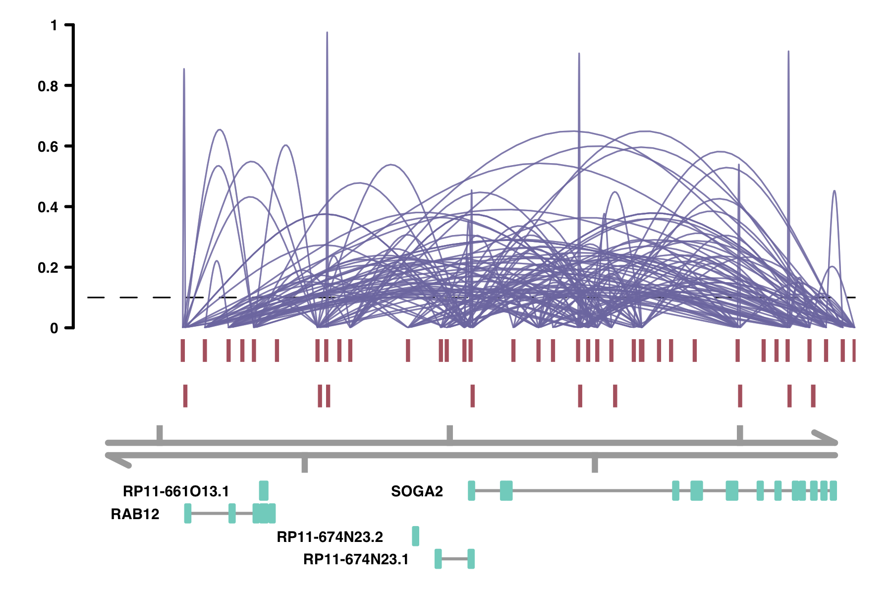
plot_connections(conns, "chr18", 8575097, 8839855,
gene_model = gene_annotation_sample,
coaccess_cutoff = .25,
connection_width = .5,
collapseTranscripts = "longest" )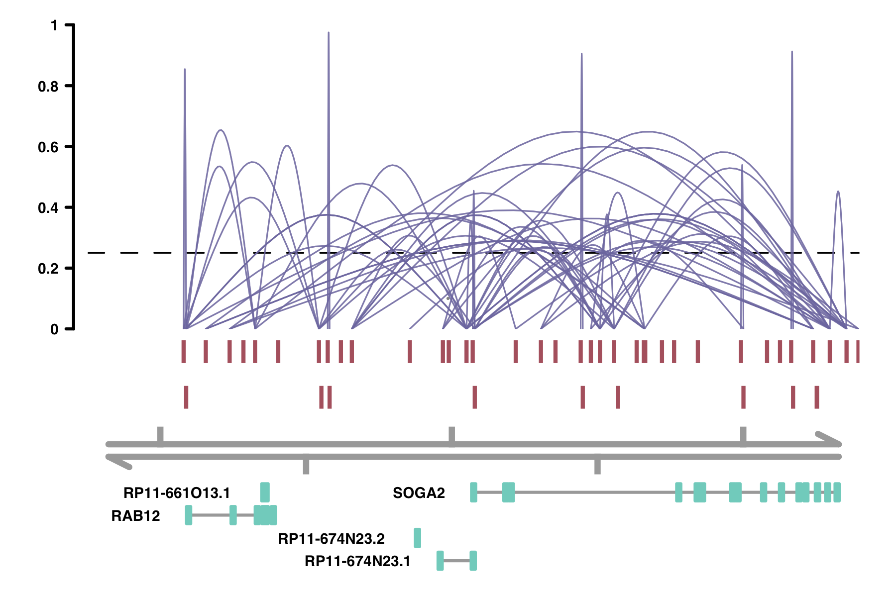
Comparing Cicero connections to other datasets
Often, it is useful to compare Cicero connections to other datasets with similar kinds of connections. For
example, you might want to compare the output of Cicero to ChIA-PET ligations. To do this, Cicero includes a
function called compare_connections. This function takes as input two data frames of connection
pairs, conns1 and conns2, and returns a logical vector of connections from
conns1 found in conns2. The comparison in this function is conducted using the
GenomicRanges
package, and uses the max_gap argument from that package to allow slop in the comparisons.
For example, if we wanted to compare our Cicero predictions to a set of (made-up) ChIA-PET connections, we could run:
chia_conns <-  data.frame(Peak1 = c("chr18_10000_10200", "chr18_10000_10200",
                                  "chr18_49500_49600"),
                        Peak2 = c("chr18_10600_10700", "chr18_111700_111800",
                                  "chr18_10600_10700"))
head(chia_conns)

#               Peak1               Peak2
# 1 chr18_10000_10200   chr18_10600_10700
# 2 chr18_10000_10200 chr18_111700_111800
# 3 chr18_49500_49600   chr18_10600_10700

conns$in_chia <- compare_connections(conns, chia_conns)

head(conns)

#               Peak1               Peak2    coaccess in_chia
# 2 chr18_10025_10225   chr18_10603_11103  0.85209126    TRUE
# 3 chr18_10025_10225   chr18_11604_13986 -0.55433268   FALSE
# 4 chr18_10025_10225   chr18_49557_50057 -0.43594546   FALSE
# 5 chr18_10025_10225   chr18_50240_50740 -0.43662436   FALSE
# 6 chr18_10025_10225 chr18_104385_104585  0.00000000   FALSE
# 7 chr18_10025_10225 chr18_111867_112367  0.01405174   FALSE
You may find that this overlap is too strict when comparing completely distinct datasets. Looking carefully,
the 2nd line of the ChIA-PET data matches fairly closely to the last line shown of conns. The difference is
only ~67 base pairs, which could be a matter of peak-calling. This is where the max_gap
parameter can be useful:
conns$in_chia_100 <- compare_connections(conns, chia_conns, maxgap=100)

head(conns)

#               Peak1               Peak2    coaccess in_chia in_chia_100
# 2 chr18_10025_10225   chr18_10603_11103  0.85209126    TRUE        TRUE
# 3 chr18_10025_10225   chr18_11604_13986 -0.55433268   FALSE       FALSE
# 4 chr18_10025_10225   chr18_49557_50057 -0.43594546   FALSE       FALSE
# 5 chr18_10025_10225   chr18_50240_50740 -0.43662436   FALSE       FALSE
# 6 chr18_10025_10225 chr18_104385_104585  0.00000000   FALSE       FALSE
# 7 chr18_10025_10225 chr18_111867_112367  0.01405174   FALSE        TRUE
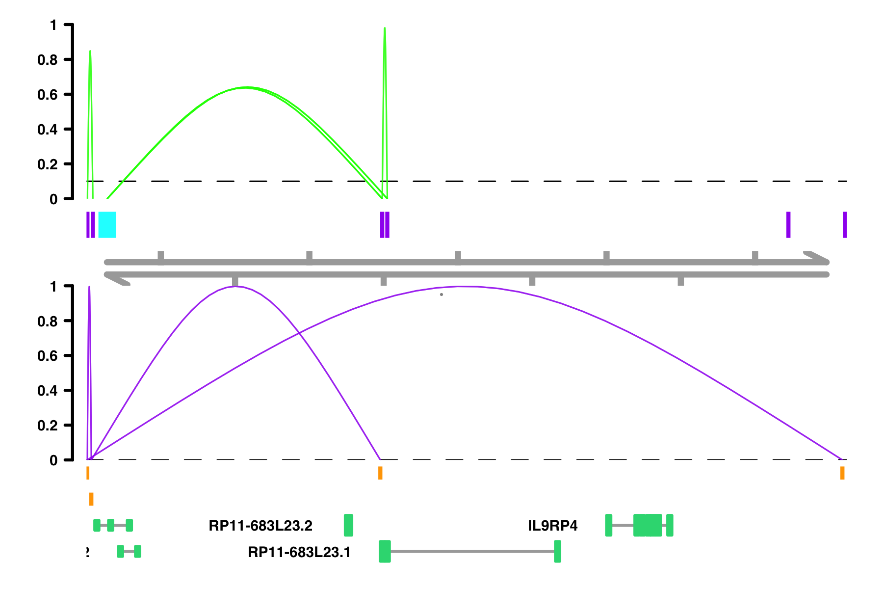
In addition, Cicero's plotting function has a way to compare datasets visually. To do this, use the
comparison_track argument. The comparison data frame must include a third
columns beyond the first two peak columns called "coaccess". This is how the plotting function determines the
height of the plotted connections. This could be a quantitative measure, like the number of ligations in
ChIA-PET, or simply a column of 1s. More info on plotting options in manual pages
?plot_connections and in the Advanced
Visualization section.
# Add a column of 1s called "coaccess"
chia_conns <-  data.frame(Peak1 = c("chr18_10000_10200", "chr18_10000_10200",
                                  "chr18_49500_49600"),
                        Peak2 = c("chr18_10600_10700", "chr18_111700_111800",
                                  "chr18_10600_10700"),
                        coaccess = c(1, 1, 1))
plot_connections(conns, "chr18", 10000, 112367,
                gene_model = gene_annotation_sample,
                coaccess_cutoff = 0,
                connection_width = .5,
                comparison_track = chia_conns,
                include_axis_track = F,
collapseTranscripts = "longest") 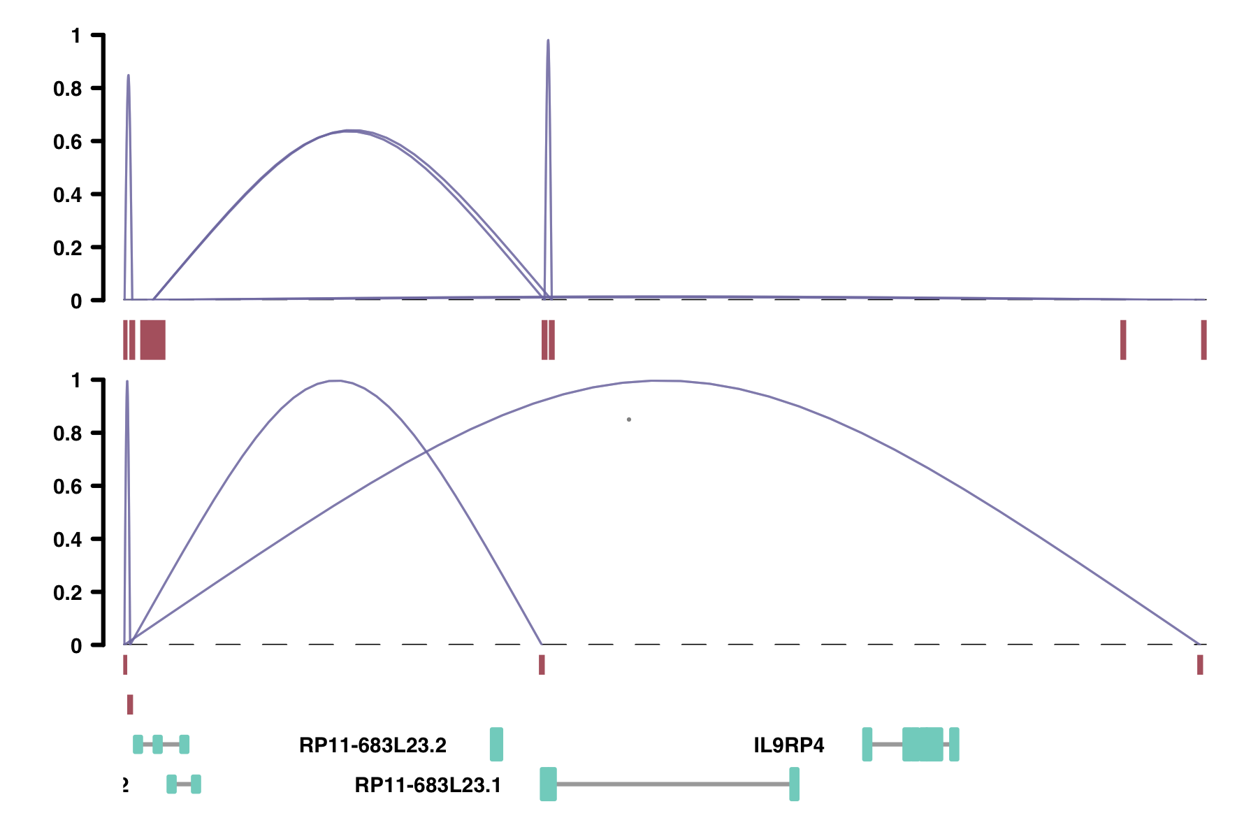
Finding cis-Co-accessibility Networks (CCANS)
In addition to pairwise co-accessibility scores, Cicero also has a function to find Cis-Co-accessibility
Networks (CCANs), which are modules of sites that are highly co-accessible with one another. We use the
Louvain community detection algorithm (Blondel et al., 2008) to find clusters of sites that tended to be
co-accessible. The function generate_ccans takes as input a connection data frame and outputs a
data frame with CCAN assignments for each input peak. Sites not included in the output data frame were not
assigned a CCAN.
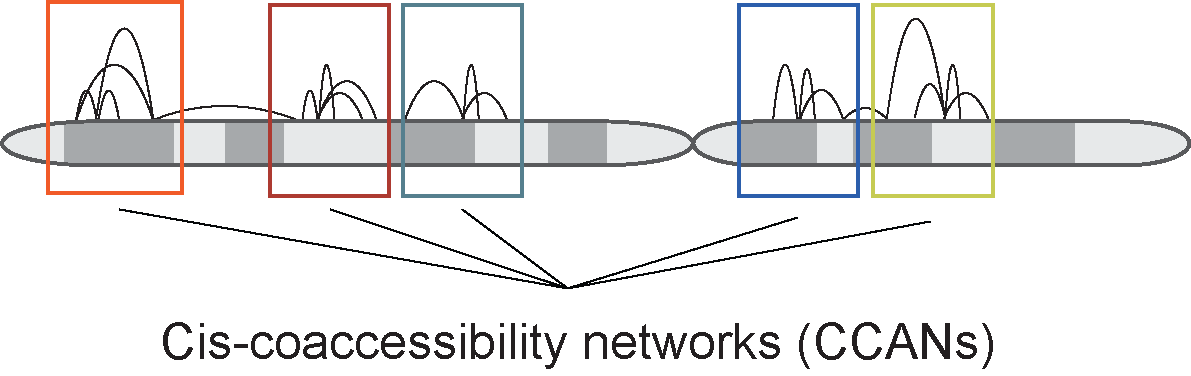
The function generate_ccans has one optional input called coaccess_cutoff_override.
When coaccess_cutoff_override is NULL, the function will determine and report an appropriate
co-accessibility score cutoff value for CCAN generation based on the number of overall CCANs at varying
cutoffs. You can also set coaccess_cutoff_override to be a numeric between 0 and 1, to override
the cutoff-finding part of the function. This option is useful if you feel that the cutoff found
automatically was too strict or loose, or for speed if you are rerunning the code and know what the cutoff
will be, since the cutoff finding procedure can be slow.
CCAN_assigns <- generate_ccans(conns)

# [1] "Co-accessibility cutoff used: 0.24"

head(CCAN_assigns)

#                                    Peak CCAN
# chr18_10025_10225     chr18_10025_10225    1
# chr18_10603_11103     chr18_10603_11103    1
# chr18_11604_13986     chr18_11604_13986    1
# chr18_49557_50057     chr18_49557_50057    1
# chr18_50240_50740     chr18_50240_50740    1
# chr18_157883_158536 chr18_157883_158536    1
Cicero gene activity scores
We have found that often, accessibility at promoters is a poor predictor of gene expression. However, using Cicero links, we are able to get a better sense of the overall accessibility of a promoter and it's associated distal sites. This combined score of regional accessibility has a better concordance with gene expression. We call this score the Cicero gene activity score, and it is calculated using two functions.
The initial function is called build_gene_activity_matrix. This function takes an input CDS and
a Cicero connection list, and outputs an unnormalized table of gene activity scores.
IMPORTANT: the input CDS must have a column in the fData table called "gene" which indicates
the gene if that peak is a promoter, and NA if the peak is distal. One way to add this column is
demonstrated below.
The output of build_gene_activity_matrix is unnormalized. It must be normalized
using a second function called normalize_gene_activities. If you intend to compare gene
activities across different datasets of subsets of data, then all gene activity subsets should be normalized
together, by passing in a list of unnormalized matrices. If you only wish to normalized one matrix, simply
pass it to the function on its own. normalize_gene_activities also requires a named vector of
of total accessible sites per cell. This is easily found in the pData table of your CDS, called
"num_genes_expressed". See below for an example. Normalized gene activity scores range from 0 to 1.
#### Add a column for the fData table indicating the gene if a peak is a promoter ####
# Create a gene annotation set that only marks the transcription start sites of
# the genes. We use this as a proxy for promoters.
# To do this we need the first exon of each transcript
pos <- subset(gene_annotation_sample, strand == "+")
pos <- pos[order(pos$start),]
pos <- pos[!duplicated(pos$transcript),] # remove all but the first exons per transcript
pos$end <- pos$start + 1 # make a 1 base pair marker of the TSS

neg <- subset(gene_annotation_sample, strand == "-")
neg <- neg[order(neg$start, decreasing = TRUE),]
neg <- neg[!duplicated(neg$transcript),] # remove all but the first exons per transcript
neg$start <- neg$end - 1

gene_annotation_sub <- rbind(pos, neg)

# Make a subset of the TSS annotation columns containing just the coordinates
# and the gene name
gene_annotation_sub <- gene_annotation_sub[,c(1:3, 8)]

# Rename the gene symbol column to "gene"
names(gene_annotation_sub)[4] <- "gene"

input_cds <- annotate_cds_by_site(input_cds, gene_annotation_sub)

head(fData(input_cds))

#                               site_name chr    bp1    bp2 num_cells_expressed overlap          gene
# chr18_10025_10225     chr18_10025_10225  18  10025  10225                   5      NA          <NA>
# chr18_10603_11103     chr18_10603_11103  18  10603  11103                   1       1    AP005530.1
# chr18_11604_13986     chr18_11604_13986  18  11604  13986                   9     203    AP005530.1
# chr18_49557_50057     chr18_49557_50057  18  49557  50057                   2     331 RP11-683L23.1
# chr18_50240_50740     chr18_50240_50740  18  50240  50740                   2     129 RP11-683L23.1
# chr18_104385_104585 chr18_104385_104585  18 104385 104585                   1      NA          <NA>

#### Generate gene activity scores ####
# generate unnormalized gene activity matrix
unnorm_ga <- build_gene_activity_matrix(input_cds, conns)

# remove any rows/columns with all zeroes
unnorm_ga <- unnorm_ga[!Matrix::rowSums(unnorm_ga) == 0, !Matrix::colSums(unnorm_ga) == 0]

# make a list of num_genes_expressed
num_genes <- pData(input_cds)$num_genes_expressed
names(num_genes) <- row.names(pData(input_cds))

# normalize
cicero_gene_activities <- normalize_gene_activities(unnorm_ga, num_genes)

# if you had two datasets to normalize, you would pass both:
# num_genes should then include all cells from both sets
unnorm_ga2 <- unnorm_ga
cicero_gene_activities <- normalize_gene_activities(list(unnorm_ga, unnorm_ga2), num_genes)
Advanced visualizaton
Some useful parameters
Here, we will show some example of plotting parameters you may want to use to further explore your data
visually. Find documentation of all of the parameters in R's manual pages using
?plot_connections.
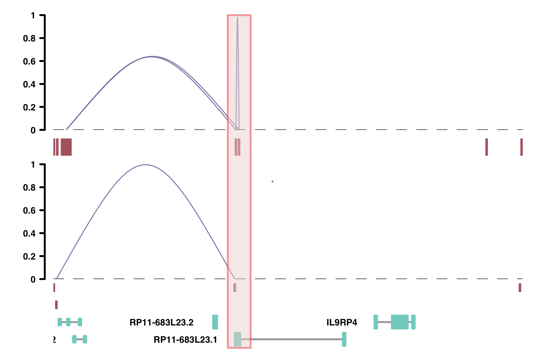
Viewpoints: the viewpoint parameter lets you view only the connections
originating from a specific place in the genome. This might be useful in comparing data with 4C-seq data.
plot_connections(conns, "chr18", 10000, 112367,
                viewpoint = "chr18_48000_53000",
                gene_model = gene_annotation_sample,
                coaccess_cutoff = 0,
                connection_width = .5,
                comparison_track = chia_conns,
                include_axis_track = F,
                collapseTranscripts = "longest")
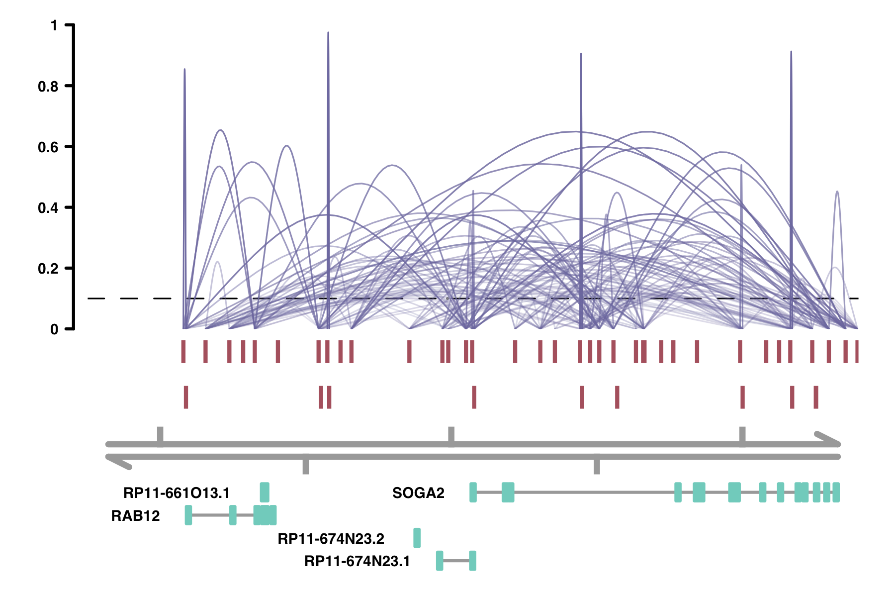
alpha_by_coaccess: the alpha_by_coaccess parameter lets you is
useful when you are concerned about overplotting. This parameter causes the alpha (transparency) of the
connection curves to be scaled based on the magnitude of the co-accessibility. Compare the following two
plots.
plot_connections(conns,
                alpha_by_coaccess = FALSE,
                "chr18", 8575097, 8839855,
                gene_model = gene_annotation_sample,
                coaccess_cutoff = 0.1,
                connection_width = .5,
                collapseTranscripts = "longest" )

plot_connections(conns,
                alpha_by_coaccess = TRUE,
                "chr18", 8575097, 8839855,
                gene_model = gene_annotation_sample,
                coaccess_cutoff = 0.1,
                connection_width = .5,
                collapseTranscripts = "longest" )
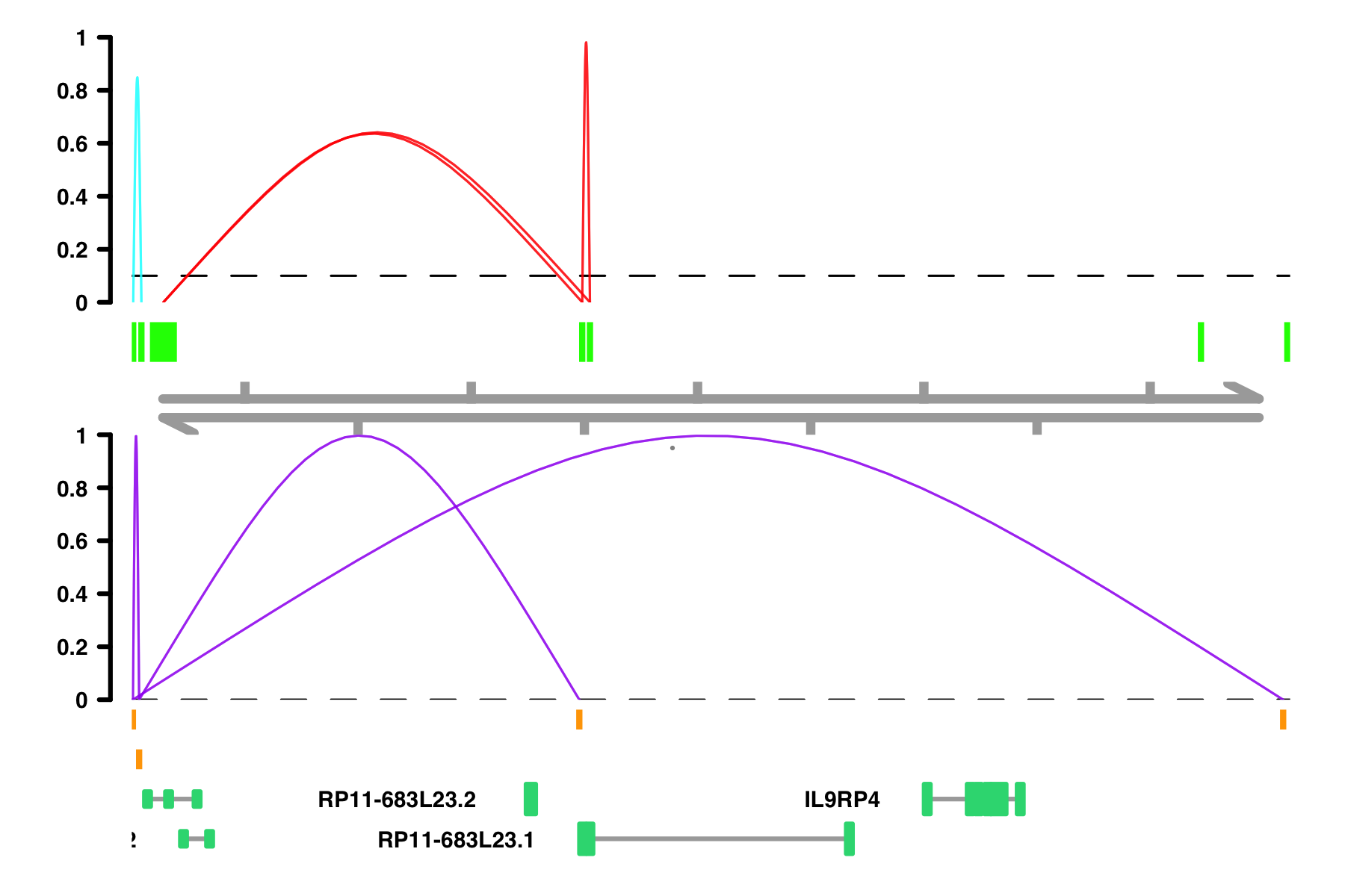
Colors: There are several parameters having to do with colors:
peak_colorcomparison_peak_colorconnection_colorcomparison_connection_colorgene_model_colorviewpoint_colorviewpoint_fill
peak_color and
comparison_peak_color, the column should correspond to Peak1 color assignment.
# When the color column is not already colors, random colors are assigned
plot_connections(conns,
                "chr18", 10000, 112367,
                connection_color = "in_chia_100",
                comparison_track = chia_conns,
                peak_color = "green",
                comparison_peak_color = "orange",
                comparison_connection_color = "purple",
                gene_model_color = "#2DD881",
                gene_model = gene_annotation_sample,
                coaccess_cutoff = 0.1,
                connection_width = .5,
                collapseTranscripts = "longest" )
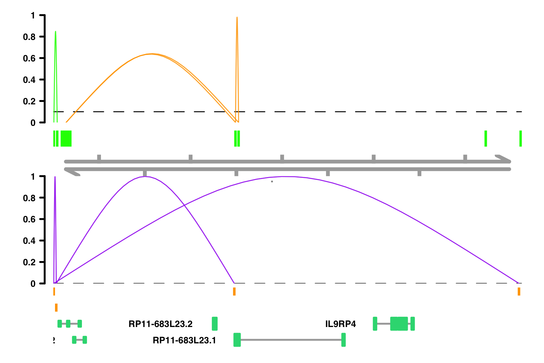
# If I want specific color scheme, I can make a column of color names
conns$conn_color <- "orange"
conns$conn_color[conns$in_chia_100] <- "green"
plot_connections(conns,
                "chr18", 10000, 112367,
                connection_color = "conn_color",
                comparison_track = chia_conns,
                peak_color = "green",
                comparison_peak_color = "orange",
                comparison_connection_color = "purple",
                gene_model_color = "#2DD881",
                gene_model = gene_annotation_sample,
                coaccess_cutoff = 0.1,
                connection_width = .5,
                collapseTranscripts = "longest" )
# For coloring Peaks, I need the color column to correspond to Peak1:
conns$peak1_color <- FALSE
conns$peak1_color[conns$Peak1 == "chr18_11604_13986"] <- TRUE
plot_connections(conns,
                "chr18", 10000, 112367,
                connection_color = "green",
                comparison_track = chia_conns,
                peak_color = "peak1_color",
                comparison_peak_color = "orange",
                comparison_connection_color = "purple",
                gene_model_color = "#2DD881",
                gene_model = gene_annotation_sample,
                coaccess_cutoff = 0.1,
                connection_width = .5,
                collapseTranscripts = "longest" )
Customizing everything with return_as_list
We realize that you may wish to plot other kinds of data along with Cicero connections. Because of this, we
include the return_as_list option. This parameter allows you to use the extensive functionality
of Gviz to plot many different
kinds of genomic data. See the
Gviz user guide
to see the many options.
If return_as_list
TRUE, an image will not be plotted, and instead, a
list of plot components will be returned. Let's go back to a simpler example:
plot_list <- plot_connections(conns,
                    "chr18", 10000, 112367,
                    gene_model = gene_annotation_sample,
                    coaccess_cutoff = 0.1,
                    connection_width = .5,
                    collapseTranscripts = "longest",
                    return_as_list = TRUE)
plot_list
# [[1]]
# CustomTrack ''

# [[2]]
# AnnotationTrack 'Peaks'
# | genome: NA
# | active chromosome: chr18
# | annotation features: 7

# [[3]]
# Genome axis 'Axis'

# [[4]]
# GeneRegionTrack 'Gene Model'
# | genome: NA
# | active chromosome: chr18
# | annotation features: 33
This made a list of components in the order of plotting. First is the CustomTrack, which is the Cicero connections, next is the peak annotation track, next is the genome axis track, and lastly is the gene model track. I can now add another track, rearrange tracks, or replace tracks using Gviz:
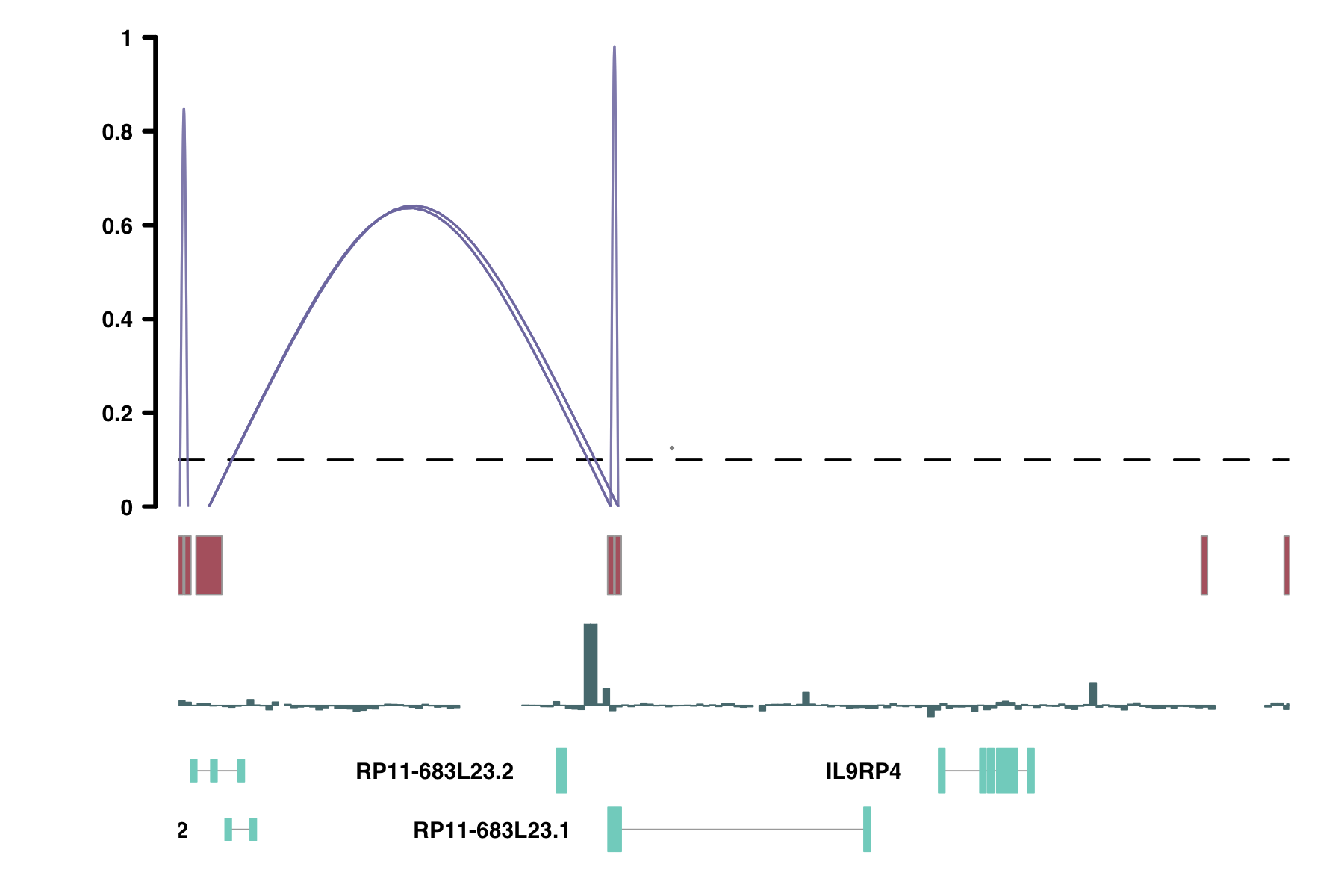
conservation <- UcscTrack(genome = "hg19", chromosome = "chr18",
                        track = "Conservation", table = "phyloP100wayAll",
                        fontsize.group=6,fontsize=6, cex.axis=.8,
                        from = 10000, to = 112367, trackType = "DataTrack",
                        start = "start", end = "end", data = "score", size = .1,
                        type = "histogram", window = "auto", col.histogram = "#587B7F",
                        fill.histogram = "#587B7F", ylim = c(-1, 2.5),
                        name = "Conservation")
# I will replace the genome axis track with a track on conservation values
plot_list[[3]] <- conservation

# To make the plot, I will now use Gviz's plotTracks function
# The included options are the defaults in plot_connections,
# but all can be modified according to Gviz's documentation

# The main new paramter that you must include, is the sizes
# parameter. This parameter controls what proportion of the
# height of your plot is allocated for each track. The sizes
# parameter must be a vector of the same length as plot_list

Gviz::plotTracks(plot_list,
                sizes = c(2,1,1,1),
                from = 10000, to = 112367, chromosome = "chr18",
                transcriptAnnotation = "symbol",
                col.axis = "black",
                fontsize.group = 6,
                fontcolor.legend = "black",
                lwd=.3,
                title.width = .5,
                background.title = "transparent",
                col.border.title = "transparent")
Important Considerations for Non-Human Data
Cicero's default parameters were designed for use in human and mouse. There are a few parameters that we expect will need to be changed for use in different model organisms. Here are the parameters along with a brief discussion of each:
Parameters to consider for non-human data
| Parameter | Functions where used | Notes | Potential values |
|---|---|---|---|
s |
estimate_distance_parameter, generate_cicero_models |
As discussed previously, the value s is the scaling exponent of the power-law
function that estimates the global decay in contact frequency. This value is generally estimated
using Hi-C contact frequencies. As a default, we have used 0.75, which corresponds to the
“tension globule” polymer model of DNA (Sanborn et al., 2015). However, in other organisms,
different decay functions have been observed. For example, in Drosophila, a scaling value of 0.85
has been proposed (Sexton et al., 2012).
|
Human and mouse: 0.75 Drosophila: 0.85 |
distance_constraint |
estimate_distance_parameter |
The value distance_constraint is the distance in base pairs at beyond which few
(less than 5%) meaningful cis-regulatory connections are expected to exist. While there are
examples of very long range cis-regulatory contacts in various organisms, this value should be
more of a general rule as Cicero can still detect longer range connections with high
co-accessibility.
|
Human and mouse: 250,000 Drosophila: 50,000 |
window |
estimate_distance_parameter, generate_cicero_models |
The window value is the length in base pairs of the sliding window that Cicero
will use when measuring co-accessibility. This value must be significantly longer (>30%) than
the value for distance_constraint. This is the maximum distance of sites that
will be compared.
|
Human and mouse: 500,000 Drosophila: 100,000 |
Single-cell accessibility trajectories
The second major function of the Cicero package is to extend Monocle 2 for use with single-cell accessibility data. The main obstacle to overcome with chromatin accessibility data is the sparsity, so most of the extensions and methods are designed to address that.
Constructing trajectories with accessibility data
We strongly recommend that you consult the Monocle website, especially this section prior to reading about Cicero's extension of the Monocle analysis described. Briefly, Monocle infers pseudotime trajectories in three steps:
- Choosing sites that define progress
- Reducing the dimensionality of the data
- Ordering cells in pseudotime
Aggregation: the primary method for addressing sparsity
The primary way that the Cicero package deals with the sparsity of single-cell chromatin accessibility data is through aggregation. Aggregating the counts of either single cells or single peaks allows us to produce a "consensus" count matrix, reducing noise and allowing us to move out of the binary regime. Under this grouping, the number of cells in which a particular site is accessible can be modeled with a binomial distribution or, for sufficiently large groups, the corresponding Gaussian approximation. Modeling grouped accessibility counts as normally distributed allows Cicero to easily adjust them for arbitrary technical covariates by simply fitting a linear model and taking the residuals with respect to it as the adjusted accessibility score for each group of cells. We demonstrate how to apply this grouping practically below.
aggregate_nearby_peaks
The primary aggregation used for trajectory reconstruction is betweeen nearby peaks. This keeps single cells
separate while aggregating regions of the genome and looking for chromatin accessibility within them. The
function aggregate_nearby_peaks finds sites within a certain distance of each other and
aggregates them together by summing their counts. Depending on the density of your data, you may want to try
different distance parameters. In published work we have used 1000 and 10,000.
data("cicero_data")
input_cds <- make_atac_cds(cicero_data, binarize = TRUE)

# Add some cell meta-data
data("cell_data")
pData(input_cds) <- cbind(pData(input_cds), cell_data[row.names(pData(input_cds)),])
pData(input_cds)$cell <- NULL

agg_cds <- aggregate_nearby_peaks(input_cds, distance = 10000)
agg_cds <- detectGenes(agg_cds)
agg_cds <- estimateSizeFactors(agg_cds)
agg_cds <- estimateDispersions(agg_cds)
Choosing sites that define progress
There are several options for choosing the sites to use during dimensionality reduction. Monocle has a discussion about the options here. Any of these options could be used with your new aggregated CDS, depending on the information you have a available in your dataset. Here, we will show two examples:
Choose sites by differential analysisAlternative
If your data has defined beginning and end points, you can determine which sites define progress by a
differential accessibility test. We use Monocle's differentialGeneTest function looking for
sites that are different in the timepoint groups.
# This takes a few minutes to run
diff_timepoint <- differentialGeneTest(agg_cds,
                    fullModelFormulaStr="~timepoint + num_genes_expressed")

# We chose a very high q-value cutoff because there are
# so few sites in the sample dataset, in general a q-value
# cutoff in the range of 0.01 to 0.1 would be appropriate
ordering_sites <- row.names(subset(diff_timepoint, qval < 1))
Choose sites by dpFeature Alternative
Alternatively, you can choose sites for dimensionality reduction by using Monocle's dpFeature method. dpFeature chooses sites based on how they differ among clusters of cells. Here, we give some example code reproduced from Monocle, for more information, see the Monocle description.
plot_pc_variance_explained(agg_cds, return_all = F) #Choose 2 PCs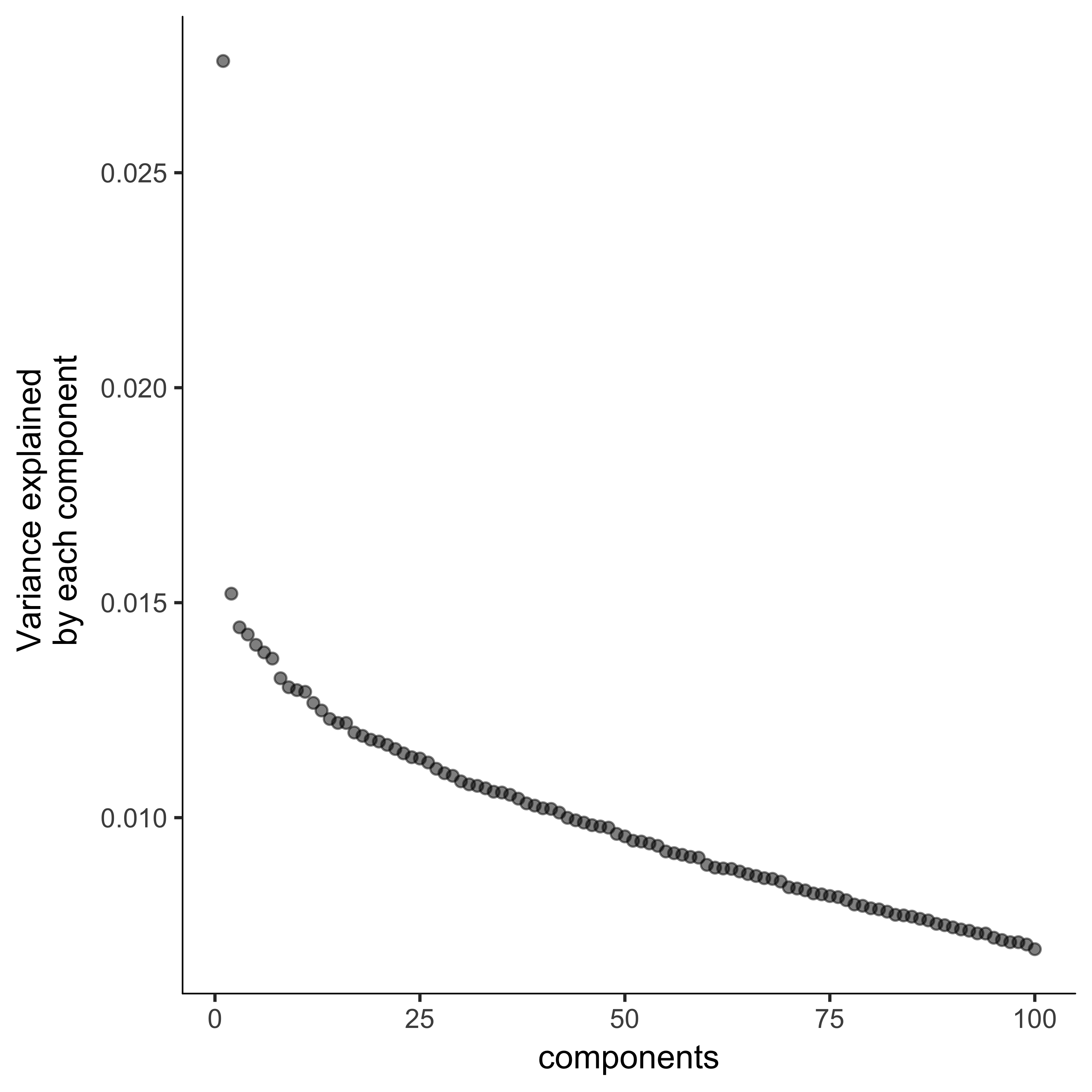
agg_cds <- reduceDimension(agg_cds,
                            max_components = 2,
                            norm_method = 'log',
                            num_dim = 3,
                            reduction_method = 'tSNE',
                            verbose = T)

agg_cds <- clusterCells(agg_cds, verbose = F)

plot_cell_clusters(agg_cds, color_by = 'as.factor(Cluster)')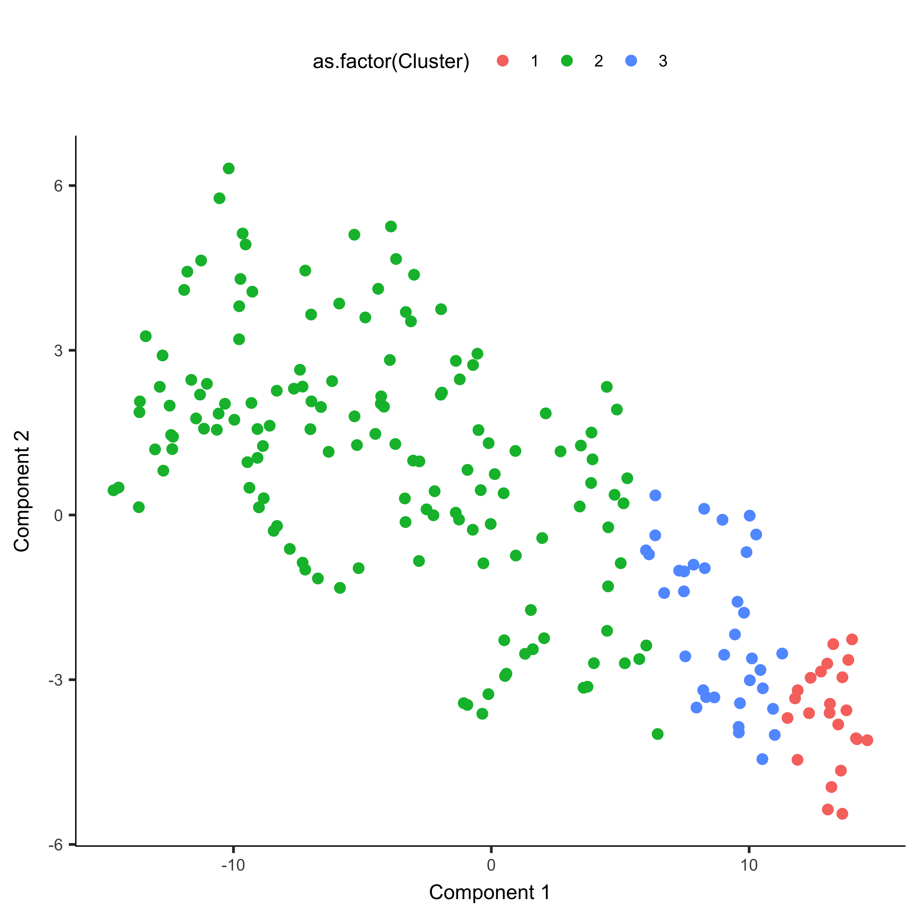
clustering_DA_sites <- differentialGeneTest(agg_cds, #Takes a few minutes
                                          fullModelFormulaStr = '~Cluster')

ordering_sites <-
row.names(clustering_DA_sites)[order(clustering_DA_sites$qval)][1:1000]
Reduce the dimensionality of the data and order cells
However you chose your ordering sites, the first step of dimensionality reduction is to use
setOrderingFilter to mark the sites you want to use for dimesionality reduction. In the
following figures, we are using the ordering_sites from
Choose sites by differential analysis above.
agg_cds <- setOrderingFilter(agg_cds, ordering_sites)Next, we use DDRTree to reduce dimensionality and then order the cells along the trajectory. Importantly, we use num_genes_expressed in our residual model formula to account for overall assay efficiency.
agg_cds <- reduceDimension(agg_cds, max_components = 2,
        residualModelFormulaStr="~as.numeric(num_genes_expressed)",
        reduction_method = 'DDRTree')
agg_cds <- orderCells(agg_cds)
plot_cell_trajectory(agg_cds, color_by = "timepoint")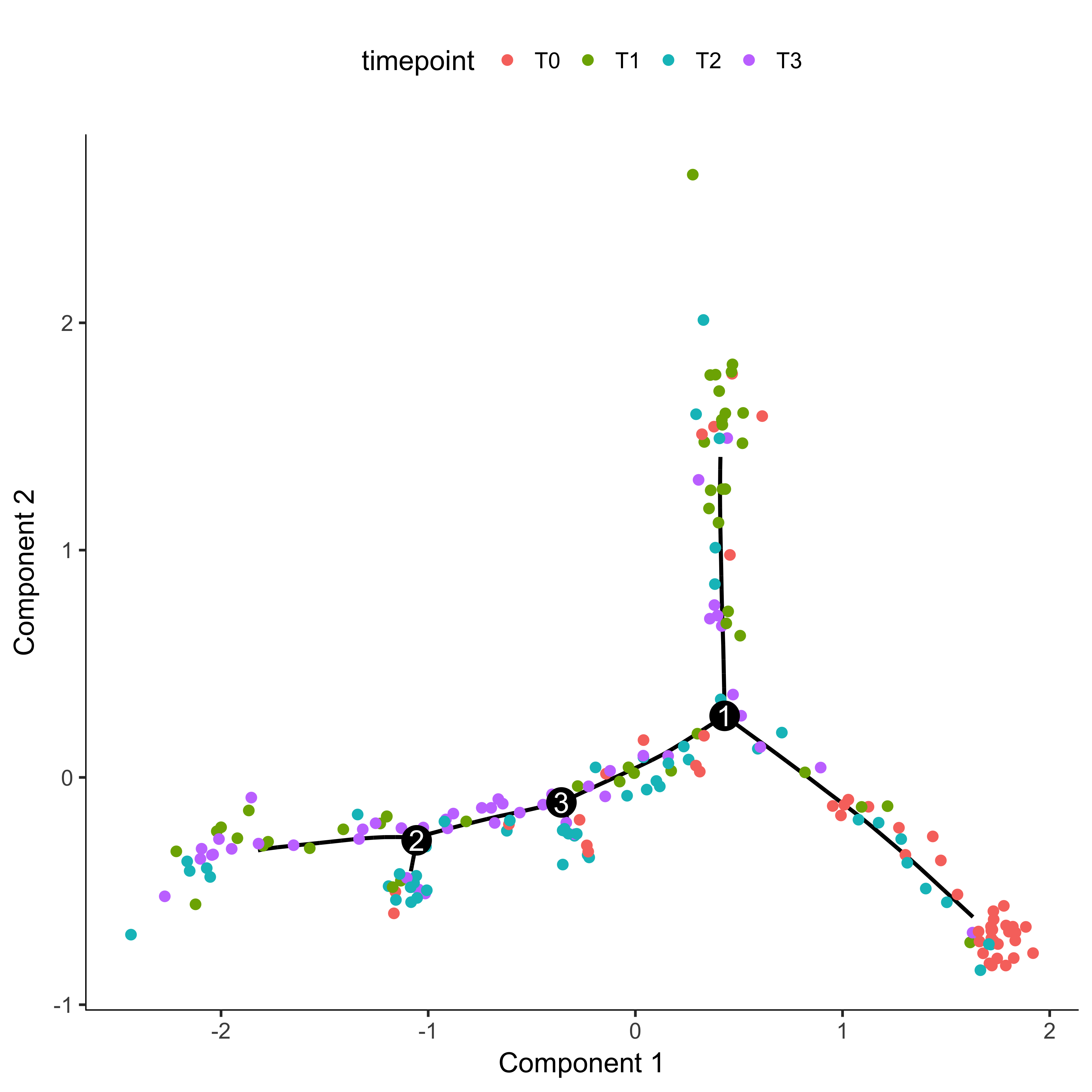
Once you have a cell trajectory, you need to make sure that pseudotime proceeds how you expect. In our example, we want pseudotime to start where most of the time 0 cells are located and proceed towards the later timepoints. Further information on this can be found here on the Monocle website. We first color our trajectory plot by State, which is how Monocle assigns segments of the tree.
plot_cell_trajectory(agg_cds, color_by = "State")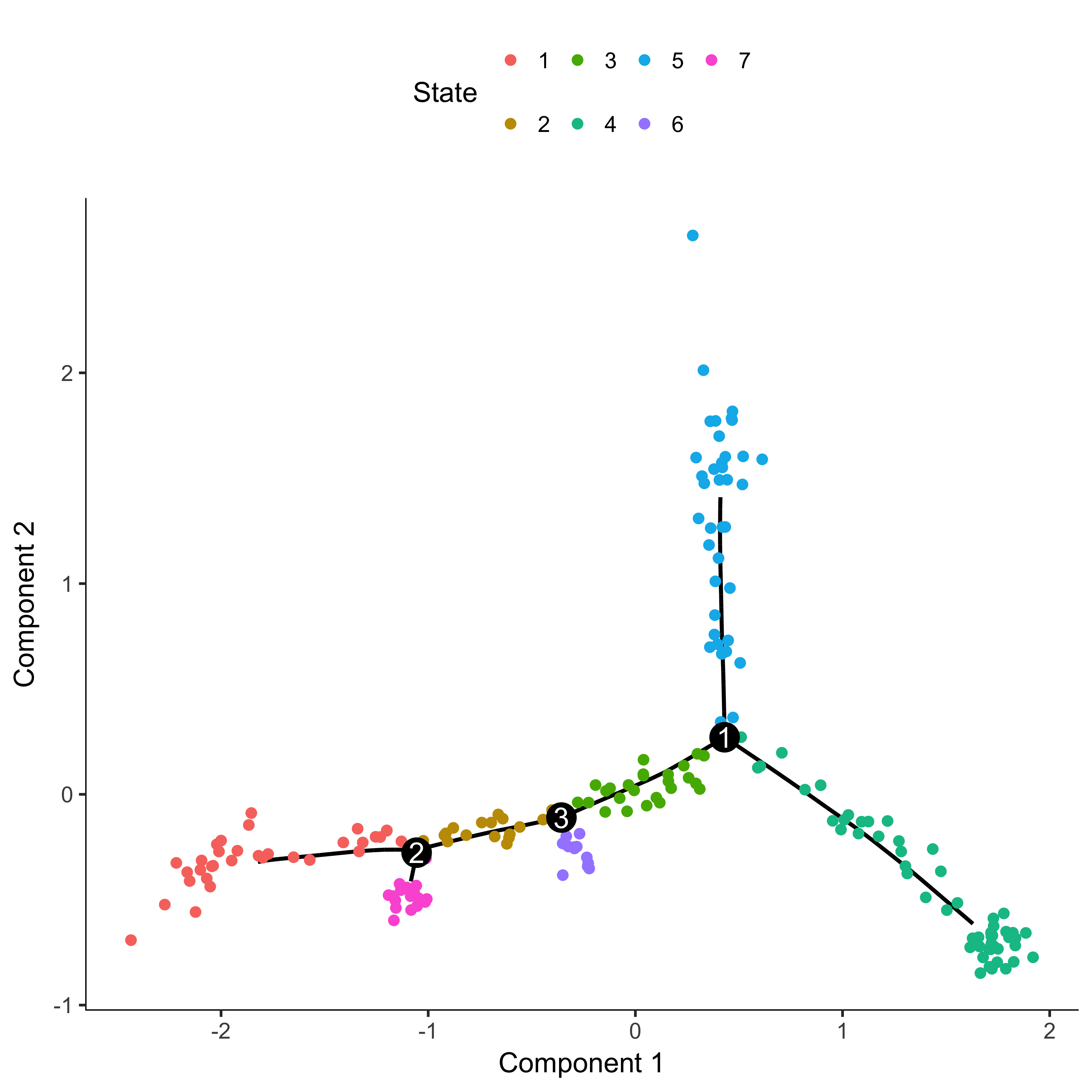
From this plot, we can see that the beginning of pseudotime should be from state 4. We now reorder cells setting the root state to 4. We can then check that the ordering makes sense by coloring the plot by Pseudotime.
agg_cds <- orderCells(agg_cds, root_state = 4)
plot_cell_trajectory(agg_cds, color_by = "Pseudotime")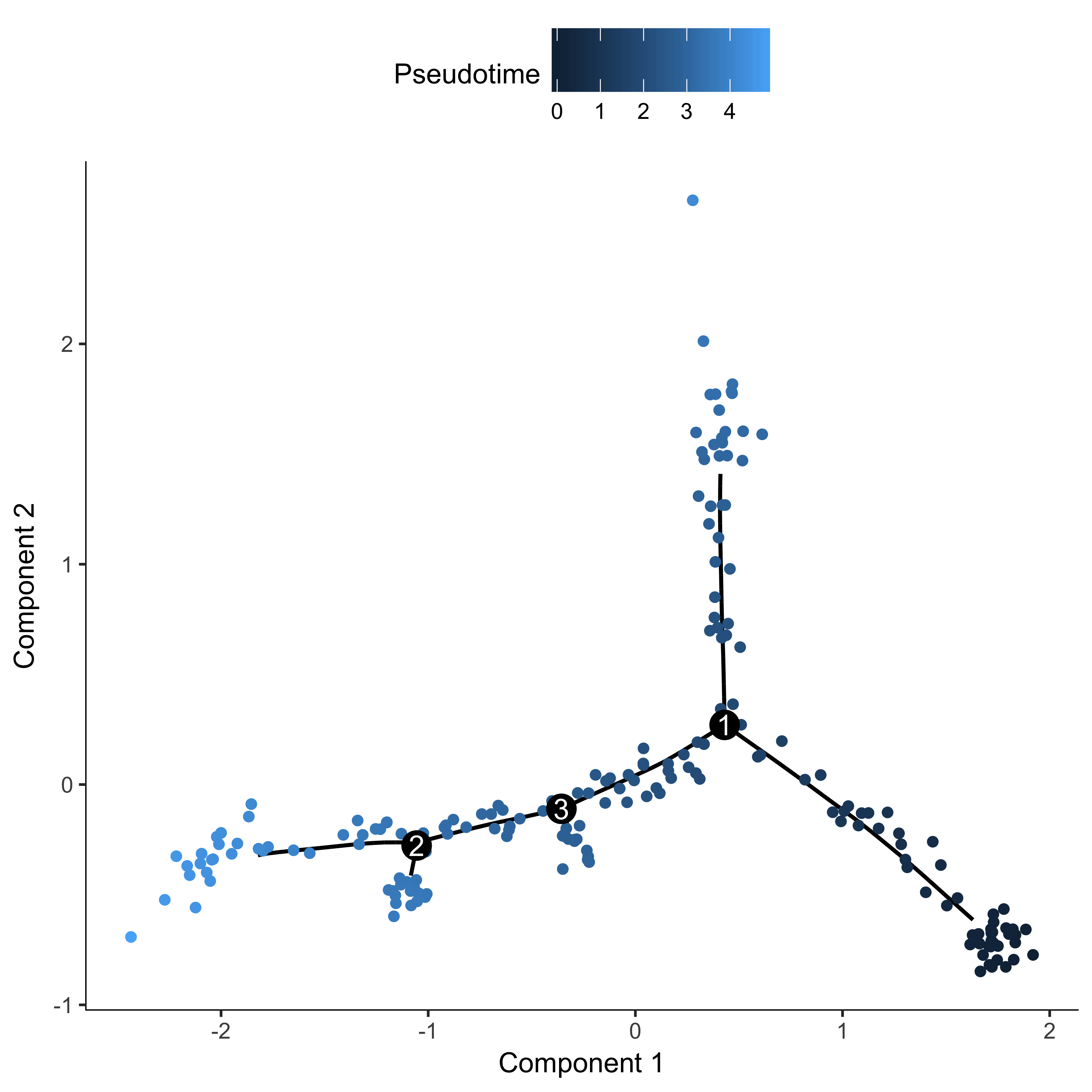
Now that we have Pseudotime values for each cell (pData(agg_cds)$Pseudotime), we need to assign
these values back to our original CDS object. In addition, we will assign the State information back to the
original CDS.
pData(input_cds)$Pseudotime <- pData(agg_cds)[colnames(input_cds),]$Pseudotime
pData(input_cds)$State <- pData(agg_cds)[colnames(input_cds),]$State
Differential Accessibility Analysis
Once you have your cells ordered in pseudotime, you can ask where in the genome chromatin accessibility is changing across time. If you know of specific sites that are important to your system, you may want to visualize the accessibility at those sites across pseudotime.
Visualizing accessibility across pseudotime
plot_accessibility_in_pseudotime
For simplicity, we will exclude the branch in our trajectory to make our trajectory linear.
input_cds_lin <- input_cds[,row.names(subset(pData(input_cds), State  != 5))]

plot_accessibility_in_pseudotime(input_cds_lin[c("chr18_38156577_38158261", "chr18_48373358_48374180", "chr18_60457956_60459080")])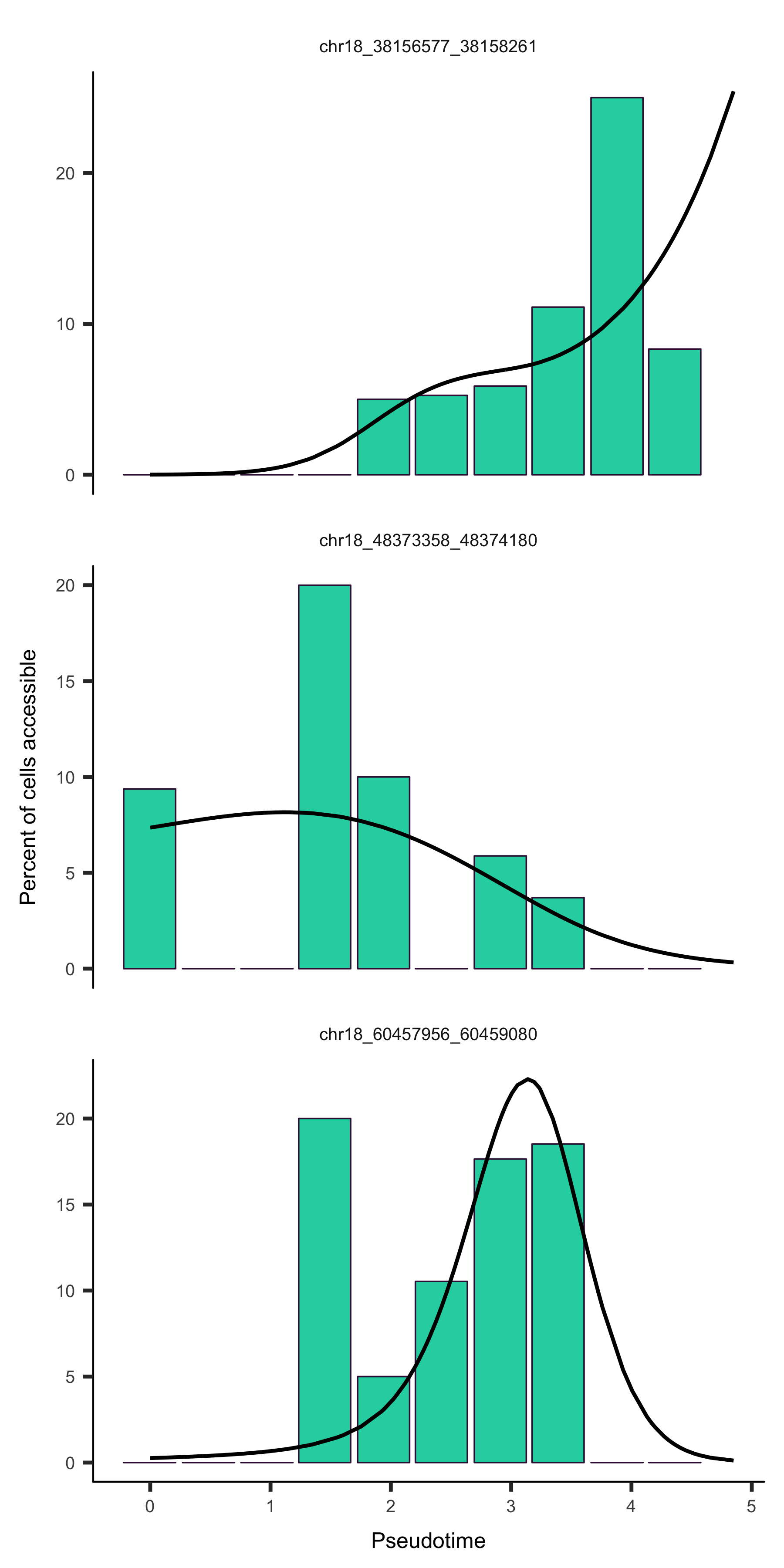
Running differentialGeneTest with single cell chromatin accessibility data
In the previous section, we used aggregation of sites to discover cell-level information (cell pseudotime).
In this section, we are interested in a site-level statistic (whether a site is changing in pseudotime), so
we will aggregate similar cells. To do this, Cicero has a useful function called
aggregate_by_cell_bin.
aggregate_by_cell_bin
We use the function aggregate_by_cell_bin to aggregate our input CDS object by a column in the
pData table. In this example, we will assign cells to bins by cutting the pseudotime trajectory into 10 parts.
pData(input_cds_lin)$cell_subtype <- cut(pData(input_cds_lin)$Pseudotime, 10)
binned_input_lin <-aggregate_by_cell_bin(input_cds_lin, "cell_subtype")
We are now ready to run Monocle's differentialGeneTest function to find sites that are differentially accessible across pseudotime. In this example, we include num_genes_expressed as a covariate to subtract its effect.
diff_test_res <- differentialGeneTest(binned_input_lin,
  fullModelFormulaStr="~sm.ns(Pseudotime, df=3) + sm.ns(num_genes_expressed, df=3)",
  reducedModelFormulaStr="~sm.ns(num_genes_expressed, df=3)", cores=1)
Useful Functions
annotate_cds_by_site
It is often useful to add additional annotations about your peaks to your CDS object. For example, you might
want to know which peaks overlap an exon, or a transcription start site. Cicero includes the function
annotate_cds_by_site, which takes as input your CDS, and a data frame or file path with
bed-format information (chromosome, bp1, bp2, further columns). For example, suppose I have some data
(feat) about epigenetic marks in my system:
head(fData(input_cds))

#                               site_name chr    bp1    bp2 num_cells_expressed
# chr18_10025_10225     chr18_10025_10225  18  10025  10225                   5
# chr18_10603_11103     chr18_10603_11103  18  10603  11103                   1
# chr18_11604_13986     chr18_11604_13986  18  11604  13986                   9
# chr18_49557_50057     chr18_49557_50057  18  49557  50057                   2
# chr18_50240_50740     chr18_50240_50740  18  50240  50740                   2
# chr18_104385_104585 chr18_104385_104585  18 104385 104585                   1

feat <- data.frame(chr = c("chr18", "chr18", "chr18", "chr18"),
                  bp1 = c(10000, 10800, 50000, 100000),
                  bp2 = c(10700, 11000, 60000, 110000),
                  type = c("Acetylated", "Methylated", "Acetylated", "Methylated"))
head(feat)
#     chr    bp1    bp2       type
# 1 chr18  10000  10700 Acetylated
# 2 chr18  10800  11000 Methylated
# 3 chr18  50000  60000 Acetylated
# 4 chr18 100000 110000 Methylated
I can use annotate_cds_by_site to determine which of my peaks have those epigenetic marks.
temp <- annotate_cds_by_site(input_cds, feat)
head(fData(temp))

#                               site_name chr    bp1    bp2 num_cells_expressed overlap       type
# chr18_10025_10225     chr18_10025_10225  18  10025  10225                   5     201 Acetylated
# chr18_10603_11103     chr18_10603_11103  18  10603  11103                   1     201 Methylated
# chr18_11604_13986     chr18_11604_13986  18  11604  13986                   9      NA       <NA>
# chr18_49557_50057     chr18_49557_50057  18  49557  50057                   2      58 Acetylated
# chr18_50240_50740     chr18_50240_50740  18  50240  50740                   2     501 Acetylated
# chr18_104385_104585 chr18_104385_104585  18 104385 104585                   1     201 Methylated
This function has added two columns compared to above. Overlap represents the number of base pairs
overlapping between the interval in feat and the given peak, and type is the assigned status
based on the overlap. If you look closely, site chr18_10603_11103 was actually overlapped by two
intervals in feat. In its default mode, annotate_cds_by_site will choose the
largest overlapping interval to report. If you would like to see all overlapping intervals, you can set the
all flag to TRUE.
temp <- annotate_cds_by_site(input_cds, feat, all=TRUE)
head(fData(temp))

#                               site_name chr    bp1    bp2 num_cells_expressed overlap                  type
# chr18_10025_10225     chr18_10025_10225  18  10025  10225                   5     201            Acetylated
# chr18_10603_11103     chr18_10603_11103  18  10603  11103                   1  98,201 Acetylated,Methylated
# chr18_11604_13986     chr18_11604_13986  18  11604  13986                   9      NA                  <NA>
# chr18_49557_50057     chr18_49557_50057  18  49557  50057                   2      58            Acetylated
# chr18_50240_50740     chr18_50240_50740  18  50240  50740                   2     501            Acetylated
# chr18_104385_104585 chr18_104385_104585  18 104385 104585                   1     201            Methylated
As you see above, when all is set to TRUE, all of the intervals that overlap are
reported.
find_overlapping_coordinates
Lastly, you may simply want to know which of your peaks overlap a specific region of the genome. For that
Cicero includes the function find_overlapping_coordinates.
find_overlapping_coordinates(fData(temp)$site_name, "chr18:10,100-10,604")

# [1] "chr18_10025_10225" "chr18_10603_11103"
Frequently Asked Questions
Where do I get a genome_coordinates file for my genome/build?
The genome_coordinates files are simply a table for chromosomes and their sizes. You can find one for your genome/build on the USCS genome browser website. Go here, find the "Full Data Set" link for your genome of interest, and find the [genome].chrom.sizes file. Download this and pass the path into the cicero function you're running! Note: some genomes have a lot of non-standard chromosomes in the sizes file (chr_unk, alternative haplotypes, etc). You may want to remove these lines from your file, which will help speed up your run.
Where do I get the gene_model/gene_annotation_sample for my genome/build?
A gene_model to pass to plotting functions can be derived from the ENSEMBL GTF for your
organism/build. Download the GTF file from here - found
under the "Gene sets" column. GTF files need a bit of processing to be ready for plotting:
# load in your data using rtracklayer
gene_anno <- rtracklayer::readGFF("Path/To/Downloaded/GTF.GTF")

# rename some columns to match plotting requirements
gene_anno$chromosome <- paste0("chr", gene_anno$seqid)
gene_anno$gene <- gene_anno$gene_id
gene_anno$transcript <- gene_anno$transcript_id
gene_anno$symbol <- gene_anno$gene_name
Citation
If you use Cicero to analyze your experiments, please cite:citation("cicero")
# Hannah A. Pliner, Jay Shendure & Cole Trapnell et. al. (2018). Cicero
# Predicts cis-Regulatory DNA Interactions from Single-Cell Chromatin
# Accessibility Data. Molecular Cell, 71, 858 - 871.e8.
# A BibTeX entry for LaTeX users is
# @Article{,
# title = {Cicero Predicts cis-Regulatory DNA Interactions from Single-Cell Chromatin Accessibility Data},
# journal = {Molecular Cell},
# volume = {71},
# number = {5},
# pages = {858 - 871.e8},
# year = {2018},
# issn = {1097-2765},
# doi = {https://doi.org/10.1016/j.molcel.2018.06.044},
# author = {Hannah A. Pliner and Jonathan S. Packer and José L. McFaline-Figueroa and
# Darren A. Cusanovich and Riza M. Daza and Delasa Aghamirzaie and Sanjay Srivatsan
# and Xiaojie Qiu and Dana Jackson and Anna Minkina and Andrew C. Adey and Frank J.
# Steemers and Jay Shendure and Cole Trapnell},
# }
Acknowledgements
Cicero was developed by Hannah Pliner in Cole Trapnell's and Jay Shendure's labs.This vignette was created from Wolfgang Huber's Bioconductor vignette style document, and patterned after the vignette for DESeq, by Simon Anders and Wolfgang Huber.
References
Blondel, V.D., Guillaume, J.-L., Lambiotte, R., and Lefebvre, E. (2008). Fast unfolding of communities in large networks.
Dekker, J., Marti-Renom, M.A., and Mirny, L.A. (2013). Exploring the three-dimensional organization of genomes: interpreting chromatin interaction data. Nat. Rev. Genet. 14, 390–403.
Sanborn, A.L., Rao, S.S.P., Huang, S.-C., Durand, N.C., Huntley, M.H., Jewett, A.I., Bochkov, I.D., Chinnappan, D., Cutkosky, A., Li, J., et al. (2015). Chromatin extrusion explains key features of loop and domain formation in wild-type and engineered genomes. . Proc. Natl. Acad. Sci. U. S. A. 112, E6456–E6465.
Sexton, T., Yaffe, E., Kenigsberg, E., Bantignies, F., Leblanc, B., Hoichman, M., Parrinello, H., Tanay, A., and Cavalli, G. (2012). Three-Dimensional Folding and Functional Organization Principles of the Drosophila Genome. . Cell 148:3, 458-472.